OTFS Modulation

Since R2024a

This example simulates a communication link that uses Orthogonal Time Frequency Space (OTFS) modulation and highlights its intercarrier interference (ICI) cancellation capabilities as compared to standard Orthogonal Frequency Division Multiplexing (OFDM) modulation. OTFS is a multicarrier modulation technique that is resilient in channel environments consisting of high-Doppler multipaths [1]. Most modern wireless systems use OFDM and suffer in high-Doppler channels due to its inability to cancel ICI. This example implements a simple OTFS transmitter and receiver, filters data through a channel with mobile scatterers, and equalizes the channel in the delay-Doppler (DD) domain using estimated channel parameters to detect the transmitted codewords.

OTFS Motivation

In high-Doppler channels, the channel characteristics change rapidly, resulting in low channel coherence times. Coherence time is inversely proportional to channel coefficient variability. OFDM has been the modulation scheme of choice for various wireless systems for many years. With OFDM, the high-Doppler channel environment requires frequent channel measurements and experiences ICI. Two drawbacks for OFDM in high-Doppler channel environments include the need for more frequent channel measurements and ICI:

• OFDM transmits data in the time-frequency (TF) domain, with each data symbol in its own orthogonal frequency subcarrier. Reference (pilot) symbols enable channel measurements but occupy a portion of the transmission bandwidth. Pilots must be transmitted frequently due to the rapidly changing channel characteristics. These pilots replace data and, as a result, reduce throughput.

• OFDM suffers from ICI in high-Doppler multipath channels when the individual paths have different frequency offsets resulting from different relative velocities of the scatterers. The frequency shifts from the different paths destroys the frequency domain orthogonality that is necessary for interference-free symbol detection.

OTFS modulation removes the need to frequently measure the channel because it transmits data in the delay-Doppler domain. This domain represents moving scatterers with delay (transmission delay) and speed (Doppler shift) relative to the receiver. Assuming a limited number of scatterers, the channel representation of the scatterers becomes a sparse matrix (the delay-Domain channel matrix is mostly zero except for a few non-zero entries that represent the scatterers). Efficient channel estimation and equalization techniques take advantage of this sparsity. In addition, if the scatterers maintain a steady velocity, the channel is quasi-stationary in the DD domain. The need for pilot transmissions decreases and the effective throughput increases.

Due to its resilience to high-Doppler channels, OTFS is being considered as a modulation candidate for 5G NR [2] and 6G [3] to meet new requirements for high-speed use cases.

OTFS Data Grid

In OTFS modulation, information symbols are mapped to an $$M$$-by-$$N$$ 2-D transmit data grid $$X_{dd}[k,l]$$ that represents the delay-Doppler domain, where $$k$$ is the delay axis index, $$k=0,1,...,M-1$$, and $$l$$ is the Doppler axis index, $$l=0,1,...,N-1$$. This grid is one OTFS symbol and each column in the grid is a subsymbol. The indices $$k$$ and $$l$$ relate to the actual delay and Doppler shift by the relationship delay = $$k/(M*df)$$ and Doppler = $$l/(N*T)$$, where $$df$$ is the subcarrier spacing in Hertz and $$T$$ is the duration of an OTFS subsymbol in seconds including any cyclic prefix. The indices $$k$$ and $$l$$ are the normalized delay and normalized Doppler shifts.

Delay-Doppler Domain

Operating in the delay-Doppler domain is similar to processing radar returns in pulse Doppler radar signal processing. Radar emits a narrowband pulse and sorts the returned echoes into range based on the time-of-arrival of the returned signal (as measured by the delay between transmission and reception) and speed based on the Doppler shift echoes. Similarly, a transmitter may send a signal to a receiver with multipath reflections much like radar echoes. Each multipath reflection may have a certain delay relative to the transmitter and a certain Doppler shift due to the reflector's movement relative to the receiver.

In the diagram below, the base station transmits a signal to the receiver located in a moving car. The two-dimensional delay-Doppler channel response $$H_{dd}$$, shown in the upper right, denotes individual paths with the respective path number. The size of the numbers and thickness of the paths are proportional to the path strength.

The direct line of sight is the reference time, denoted with a thick line at a delay of 0 samples. The car is moving towards the base station at 130 km/h, but the path has a Doppler shift index of 0 because the receiver in the car adjusts the carrier frequency to compensate for any Doppler shift effects. Path 1 denotes a reflection from a neighboring truck that is slower than the receiving car. Path 1 has a slightly longer transmission delay due to the longer distance that the signal must travel and has a negative Doppler shift since the car is slowly moving away from the truck. Path 2 is another reflection coming from an ambulance moving toward the car at a farther distance, so it has a positive Doppler, longer delay, and smaller path gain.

The effect of the multipath on a single DD grid element is shown below. $$X_{dd}$$ contains five transmitted signals and $$H_{dd}$$ is the channel response. $$Y_{dd}$$ is the 2-D convolution of $$X_{dd}$$ and $$H_{dd}$$. In OTFS, the time-limited signaling implies the convolution is circular and includes phase rotation, which is known as twisted convolution.

Delay-Doppler Domain to Time-Frequency Domain Representation

To understand how the delay-Doppler domain transforms to the time-frequency domain, you can relate the process to OFDM. The diagram below shows OTFS modulation and demodulation as a precoded OFDM modulation-demodulation system. $$M$$ is equivalent to the number of subcarriers in an OFDM symbol and $$N$$ is equivalent to the number of OFDM symbols contained in one frame.

The internal section of the diagram shows the familiar OFDM processing chain of OFDM modulator, channel, and OFDM demodulator. The Heisenberg transform and Wigner transform are generalizations of the OFDM modulator and OFDM demodulator, respectively.

First, the Inverse Symplectic Finite Fourier Transform (ISFFT) [1] transforms modulated symbols from the delay-Doppler domain $$X_{dd}$$ to the time-frequency domain $$X_{tf}$$:

$$X_{tf}[m,n]=\frac{1}{MN}\sum _{l=0}^{M-1}\sum _{k=0}^{N-1}{X}_{dd}[k,l]e^{j2\pi (\frac{nk}{N}-\frac{ml}{M})}.$$

The inner summation term is the inverse Discrete Fourier Transform (IDFT) of $$X_{dd}$$ over the Doppler axis:

$$\frac{1}{MN}\sum _{k=0}^{N-1}{X}_{dd}[k,l]e^{j\frac{2\pi nk}{N}}=\frac{1}{M}IFFT(X_{dd}^T{)}^T=X_{dt}.$$

This operation transforms $$X_{dd}$$ from the delay-Doppler domain to the delay-time domain, denoted by $$X_{dt}$$. In MATLAB ®, the DFT of an array operates on each column independently. The IDFT is applied to the transpose of $$X_{dd}$$ to operate the IDFT over the Doppler axis, then the result is transposed to bring the result back to the proper array dimension.

The outer summation in the ISFFT expression is the DFT over the delay axis:

$$\sum _{l=0}^{M-1}{X}_{dt}[m,n]e^{-j\frac{2\pi ml}{M}}=FFT(X_{dt})$$

so the ISFFT reduces to

$$X_{tf}[m,n]=\frac{1}{M}FFT(IFFT(X_{dd}^T{)}^T).$$

At this point, $$X_{tf}[m,n]$$ represents the data in the familiar time-frequency domain. The Heisenberg transform converts the transformed symbols $$X_{tf}$$ to a time-domain signal:

$$x(t)=\sum _{n=0}^{N-1}\sum _{m=0}^{M-1}{X}_{tf}[m,n]g(t-nT)e^{j2\pi m\Delta f(t-nT)}.$$

$$T$$ is the duration of one OFDM symbol. The pulse shaping filter $$g(t)$$ mitigates channel spreading caused by fractional Doppler shifts (when the Doppler frequency does not fall on a multiple of $$1/(NT)$$). When the filter is a rectangular window time-limited to 0 to $$T$$, the Heisenberg transform is simply an OFDM modulator operating over each column of $$X_{tf}$$. OTFS modulation then reduces to 2-D precoded OFDM modulation, where the precoding operation is the ISFFT. The ISFFT is an IDFT operating along the Doppler dimension to transform it to the time dimension and a DFT along the delay dimension to transform it to the frequency dimension. The Heisenberg transform is an IDFT operating along the frequency dimension [2], which is equivalent to OFDM modulation.

Inverse Zak Transform

The combination of ISFFT and Heisenberg transform can also be mathematically represented using the inverse Zak transform [4]. It combines the ISFFT and Heisenberg transform to eliminate an IDFT-DFT pair, such that the operation simplifies to an IDFT across the Doppler axis.

Recall that rectangular pulse shaping transforms the Heisenberg transform into an ordinary OFDM modulator, which is simply an IFFT over each column in $$X_{tf}$$. Then the IFFT of $$X_{tf}$$ is

$$X_{dt}=IFFT(X_{tf})=IFFT(\frac{1}{M}FFT(IFFT(X_{dd}^T{)}^T))$$

where $$X_{dt}$$ is the delay-time domain representation of the input data. Noting the IFFT-FFT combination cancels out each operation, the intermediate result is the inverse Zak transform $$X_{dt}$$:

$$X_{dt}=\frac{1}{M}IFFT(X_{dd}^T{)}^T.$$

This result is the same as was derived earlier with the ISFFT and Heisenberg transform pair. The inverse Zak transform outputs the discretized time domain samples $$x(i)$$ from the vectorized representation of $$X_{dt}[m,n]$$:

$$x(m+nM)=vec(X_{dt}[m,n]).$$

Inter-Symbol Interference (ISI) Mitigation

Insert a cyclic prefix or a sequence of zeros between OTFS subsymbols or symbols to prevent ISI, similar to how OFDM uses cyclic prefixes [4]. Zero padding (ZP) is an ISI mitigation technique that appends each OTFS subsymbol with zeros of length ZPLen samples.

Cyclic Prefix (CP) is a technique that prepends each OTFS subsymbol with the last CPLen samples of the respective subsymbol.

Reduced cyclic prefix (RCP) prepends the last CPLen samples of the OTFS symbol to the beginning of the symbol. Reduced zero padding (RZP) appends ZPLen zeros at the end of the OTFS symbol.

Simulate OTFS Over a High-Mobility Channel

Transmit a pilot signal in the delay-Doppler domain to sound a high-mobility channel and observe the channel response in the delay-Doppler domain. This example uses zero padding for demonstrating channel sounding and data transmission.

Simulation Setup

Configure the simulation parameters. For demonstrating basic OTFS concepts, let $$M$$ = 64 and $$N$$ = 30. Set the SNR to a high value to show the effects of ISI and ICI in different modulations and channel conditions.

M = 64;          % number of subcarriers
N = 30;          % number of subsymbols/frame
df = 15e3;       % make this the frequency bin spacing of LTE
fc = 5e9;        % carrier frequency in Hz
padLen = 10;     % make this larger than the channel delay spread channel in samples
padType = 'ZP';  % this example requires ZP for ISI mitigation
SNRdB = 40;

Grid Population for Channel Sounding

Create an empty array of size $$M$$-by-$$N$$ where the $$M$$ rows correspond to the delay bins and the $$N$$ columns map to the Doppler bins. To demonstrate how data in the delay-Doppler domain propagates through a high-mobility channel, place a pilot signal at grid position (1,16) to sound the channel. Leave the other grid elements empty so that the scatterer echoes will appear in the received delay-Doppler grid.

% Pilot generation and grid population
pilotBin = floor(N/2)+1;
Pdd = zeros(M,N);
Pdd(1,pilotBin) = exp(1i*pi/4); % populate just one bin to see the effect through the channel

OTFS Modulation

Modulate the DD data grid with the single pilot symbol using OTFS modulation. Use the helperOTFSmod function to operate the inverse Zak transform on the pilot grid Pdd.

% OTFS modulation
txOut = helperOTFSmod(Pdd,padLen,padType);

High-Mobility Channel

Create an AWGN high-mobility channel with stationary transmitter and mobile receiver, and moving scatterers of different delays and Doppler shifts:

• Create a line-of-sight path representing the main propagation path from a base station to the receiver with zero delay and zero normalized Doppler. The line-of-sight path has zero delay and zero Doppler since the receiver is synchronized in time and frequency to the base station.

• Create scatterer 1 delayed five samples from the receiver and moving away from the receiver with Doppler of three times the normalized Doppler.

• Create scatterer 2 delayed eight samples from the receiver and moving towards the receiver with Doppler of five times the normalized Doppler.

% Configure paths
chanParams.pathDelays      = [0  5   8  ]; % number of samples that path is delayed
chanParams.pathGains       = [1  0.7 0.5]; % complex path gain
chanParams.pathDopplers    = [0 -3   5  ]; % Doppler index as a multiple of fsamp/MN

fsamp = M*df;                % sampling frequency at the Nyquist rate
if strcmp(padType,'ZP') || strcmp(padType,'CP')
    Meff = M + padLen;       % number of samples per OTFS subsymbol
    numSamps = Meff * N;     % number of samples per OTFS symbol
    T = ((M+padLen)/(M*df)); % symbol time (seconds)
else
    Meff = M;                % number of samples per OTFS subsymbol
    numSamps = M*N + padLen; % number of samples per OTFS symbol
    T = 1/df;                % symbol time (seconds)
end
% Calculate the actual Doppler frequencies from the Doppler indices
chanParams.pathDopplerFreqs = chanParams.pathDopplers * 1/(N*T); % Hz

% Send the OTFS modulated signal through the channel
dopplerOut = dopplerChannel(txOut,fsamp,chanParams);

% Add white Gaussian noise
Es = mean(abs(pskmod(0:3,4,pi/4).^ 2));
n0 = Es/(10^(SNRdB/10));
chOut = awgn(dopplerOut,SNRdB,'measured');

Display the actual scatterer parameter delay and Doppler shift values to connect the normalized values to the actual values.

for k = 1:length(chanParams.pathDelays)
    fprintf('Scatterer %d\n',k);
    fprintf('\tDelay = %5.2f us\n', 1e6*chanParams.pathDelays(k)/(Meff*df));
    fprintf('\tRelative Doppler shift = %5.0f Hz (%5.0f km/h)\n', ...
        chanParams.pathDopplerFreqs(k), (physconst('LightSpeed')*chanParams.pathDopplerFreqs(k)/fc)*(3600/1000));
end

Scatterer 1

	Delay =  0.00 us

	Relative Doppler shift =     0 Hz (    0 km/h)

Scatterer 2

	Delay =  4.50 us

	Relative Doppler shift = -1297 Hz ( -280 km/h)

Scatterer 3

	Delay =  7.21 us

	Relative Doppler shift =  2162 Hz (  467 km/h)

OTFS Demodulation

To begin the demodulation process, the received signal vector is packed into an $$M$$-by-$$N$$ matrix $$Y_{dt}$$. The Wigner transform is the inverse of the Heisenberg transform. Because this example uses rectangular pulse shaping, the Wigner transform is simply an OFDM demodulation operation. Following the Wigner transform, the SFFT converts the time-frequency domain grid into the delay-Doppler domain.

In this example, use the more efficient Zak transform to demodulate the signal:

$$Y_{dd}[m,n]=M*FFT(Y_{dt}^T{)}^T.$$

Collect samples in an OTFS frame and demodulate the signal in the delay-Doppler domain.

% Get a sample window
rxIn = chOut(1:numSamps);

% OTFS demodulation
Ydd = helperOTFSdemod(rxIn,M,padLen,0,padType);

Delay-Doppler Channel Response

The output of the OTFS demodulated signal is the convolution of the pilot signal transmitted at (1,16) with the channel representation in the DD domain (5,-10) and (8,6). This is different than OFDM demodulation, where the OFDM demodulated signal is the Hadamard (element-by-element) product of the OFDM symbol with the frequency-domain channel coefficients.

A linear minimum mean square error (LMMSE) estimator is an estimation method that minimizes the mean square error between an observation $$Y$$ (the received signal) and the actual value $$P$$ (the known pilot signal), and is given as:

$${\underset{}{\overset{ˆ}{P}}}_{LMMSE}=\frac{Y*P^{*}}{|P{|}^2+{\sigma }_n^2}$$

where $$P^{*}$$ is the complex conjugate of $$P$$ and $${\sigma }_n^2$$ is the noise power. To estimate the channel response in the delay-Doppler domain, use LMMSE on each grid element $$Y_{dd}[k,l]$$ against the single pilot symbol $$P_{dd}$$ and compute the channel response $$H_{dd}$$.

% LMMSE channel estimate in the delay-Doppler domain
Hdd = Ydd * conj(Pdd(1,pilotBin)) / (abs(Pdd(1,pilotBin))^2 + n0);

Visualize the received DD grid with a mesh plot.

figure;
xa = 0:1:N-1;
ya = 0:1:M-1;
mesh(xa,ya,abs(Hdd));
view([-9.441 62.412]);
title('Delay-Doppler Channel Response H_{dd} from Channel Sounding');
xlabel('Normalized Doppler');
ylabel('Normalized Delay');
zlabel('Magnitude');

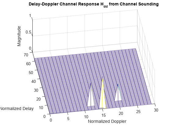
The DD grid from the channel sounding shows all the paths seen by the receiver from the single pilot, the delay of each path, the Doppler shift of each path, and the complex gain of each path. Observe how the pilot symbol convolves with the DD channel response in the delay-Doppler domain. The pilot is correctly received at the proper grid position (1,16). The other two scatterers also appear in the DD grid.

• Scatterer 1 is at grid position (1,16) + (5,-3) = (6,13).

• Scatterer 2 is at grid position (1,16) + (8,5) = (9,21).

Channel Estimation

Channel estimation in the delay-Doppler domain requires estimating the parameters (delay, Doppler, and complex gain) of all the scatterers in the channel response. From the channel response $$H_{dd}$$, find paths that exceed a preset gain threshold and store the parameters for each unique path. Store the channel estimates for later use when transmitting data over the same channel.

[lp,vp] = find(abs(Hdd) >= 0.05);
chanEst.pathGains = diag(Hdd(lp,vp));   % get path gains
chanEst.pathDelays = lp - 1;            % get delay indices
chanEst.pathDopplers = vp - pilotBin;   % get Doppler indices

Compare OFDM and OTFS in High Mobility Channels

Both OTFS and OFDM counteract the effects of ISI through cyclic prefixes. However, the single-tap frequency domain equalizer (FDE) typically used in OFDM receivers cannot undo the effects of ICI from the Doppler shifts of the different paths. In this section, form an $$M$$-by-$$N$$ grid of QPSK-mapped symbols, and transmit over a high-mobility channel using both OFDM and OTFS to compare the performance.

Generate the data for transmission.

% Data generation
Xgrid = zeros(M,N);
Xdata = randi([0,1],2*M,N);
Xgrid(1:M,:) = pskmod(Xdata,4,pi/4,InputType="bit");

OFDM Over High-Doppler Channel

In OFDM, you estimate the channel by transmitting known symbols (pilots) and measuring the distortion of the pilots at the receiver. Estimate the channel by transmitting pilots on all $$M$$ subcarriers across all $$N$$ symbols.

% Transmit pilots over all subcarriers and symbols to sound the channel
txOut = ofdmmod(exp(1i*pi/4)*ones(M,N),M,padLen);       % transmit pilots over the entire grid
dopplerOut = dopplerChannel(txOut,fsamp,chanParams);    % send through channel
chOut = awgn(dopplerOut,SNRdB,'measured');              % add noise
Yofdm = ofdmdemod(chOut(1:(M+padLen)*N),M,padLen);      % demodulate
Hofdm = Yofdm * conj(Pdd(1,pilotBin)) / (abs(Pdd(1,pilotBin))^2 + n0); % LMMSE channel estimate

Transmit the data grid using OFDM. Using the measured channel estimates, equalize using a single-tap FDE over all the symbols.

% Transmit data over the same channel and use channel estimates to equalize
txOut = ofdmmod(Xgrid,M,padLen);                        % transmit data grid

dopplerOut = dopplerChannel(txOut,fsamp,chanParams);    % send through channel
chOut = awgn(dopplerOut,SNRdB,'measured');              % add noise

rxWindow = chOut(1:(M+padLen)*N);
Yofdm = ofdmdemod(rxWindow,M,padLen);                   % demodulate

Xhat_ofdm = conj(Hofdm) .* Yofdm ./ (abs(Hofdm).^2+n0); % equalize with LMMSE

Show the received constellation. The constellation is noisy even with a high SNR. You can verify the noise is primarily from ICI by setting the Doppler shifts of the two scatterers to zero and observing that the error vector magnitude (EVM) of the constellation is reduced.

constDiagOFDM = comm.ConstellationDiagram( ...
    'ReferenceConstellation',pskmod(0:3,4,pi/4), ...
    'XLimits',[-2 2], ...
    'YLimits',[-2 2], ...
    'Title','OFDM with Single-Tap FDE');
constDiagOFDM(Xhat_ofdm(:));

XhatData = pskdemod(Xhat_ofdm,4,pi/4, ...
    OutputType="bit",OutputDataType="logical");         % decode
[~,ber] = biterr(Xdata,XhatData);
fprintf('OFDM BER with single-tap equalizer = %3.3e\n', ber);

OFDM BER with single-tap equalizer = 1.693e-02

Observe how the BER is high even with little noise. While the cyclic prefix can mitigate the ISI, single-tap equalization in the time-frequency domain cannot compensate for the ICI caused by the Doppler-shifted paths, which results in moderate BER.

OTFS Over High-Doppler Channel

Transmit the same data grid using OTFS modulation.

% OTFS modulation
txOut = helperOTFSmod(Xgrid,padLen,padType);

% Add channel and noise
dopplerOut = dopplerChannel(txOut,fsamp,chanParams);
chOut = awgn(dopplerOut,SNRdB,'measured');

A generic signal model is given as $$y=Gx+n$$, where $$x$$ and $$y$$ are the time-domain signals of length $$MN$$ transmitted into the channel and received from the time-domain channel matrix $$G$$, respectively. If $$G$$ is known, LMMSE can be used to equalize the channel [4]. In matrix form, the LMMSE is given as:

$$\underset{}{\overset{ˆ}{x}}=(G^{H}G+{\sigma }_n^2{I}_{MN}{)}^{-1}{G}^{H}y.$$

By equalizing in the time domain, you can use the information of the delay and Doppler shifts of the individual paths to remove the ICI. Form the channel matrix from the delay-Doppler channel parameter estimates found earlier.

% Form G matrix using channel estimates
G = getG(M,N,chanEst,padLen,padType);

Equalize and detect the received data using LMMSE in the delay-Doppler domain. Assume the noise power is known.

rxWindow = chOut(1:numSamps);
y_otfs = ((G'*G)+n0*eye(Meff*N)) \ (G'*rxWindow); % LMMSE

Xhat_otfs = helperOTFSdemod(y_otfs,M,padLen,0,padType); % OTFS demodulation

Show that the received constellation is cleaner than the OFDM constellation.

constDiagOTFS = comm.ConstellationDiagram( ...
    'ReferenceConstellation',pskmod(0:3,4,pi/4), ...
    'XLimits',[-2 2], ...
    'YLimits',[-2 2], ...
    'Title','OTFS with Time-Domain LMMSE Equalization');
constDiagOTFS(Xhat_otfs(:));

XhatData = pskdemod(Xhat_otfs,4,pi/4,OutputType="bit",OutputDataType="logical");
[~,ber] = biterr(Xdata,XhatData);
fprintf('OTFS BER with LMMSE equalization = %3.3e\n', ber);

OTFS BER with LMMSE equalization = 0.000e+00

OTFS is able to significantly reduce ICI.

Summary

OTFS is a promising modulation scheme to offset the effects of high Doppler in the mobile environment. This example introduces the concept of the delay-Doppler domain, the effect of the mobile channel on transmitted symbols in that domain, and how to modulate and demodulate OTFS symbols. Transmitting the same data over the same channel using OTFS and OFDM and observing their BER after simple channel estimation and equalization shows that OTFS effectively combats ICI, while OFDM cannot.

More accurate channel estimation and more efficient data detection methods are available in the literature. This example uses a simple channel estimation technique and a straightforward channel equalization method to show the merits of OTFS over OFDM in high-Doppler channels.

References

1. R. Hadani et al. "Orthogonal Time Frequency Space Modulation." 2017 IEEE Wireless Communications and Networking Conference (WCNC). San Francisco, CA, USA, 2017, pp. 1-6.

2. 3GPP TSG RA WG1. OTFS modulation waveform and reference signals for new RAT: Meeting #84-bis R1-162930. Busan, South Korea: 3GPP, 2016.

3. TSDSI. “6G Use Cases and Enabling Technologies.” Oct. 2022.

4. Y. Hong, T. Thaj, and E. Viterbo. Delay-Doppler Communications. London, Elsevier 2022.

Support Functions

function y = dopplerChannel(x,fs,chanParams)
    % Form an output vector y comprising paths of x with different
    % delays, Dopplers, and complex gains
    numPaths = length(chanParams.pathDelays);
    maxPathDelay = max(chanParams.pathDelays);
    txOutSize = length(x);
    
    y = zeros(txOutSize+maxPathDelay,1);
    
    for k = 1:numPaths
        pathOut = zeros(txOutSize+maxPathDelay,1);

        % Doppler
        pathShift = frequencyOffset(x,fs,chanParams.pathDopplerFreqs(k));
    
        % Delay and gain
        pathOut(1+chanParams.pathDelays(k):chanParams.pathDelays(k)+txOutSize) = ...
            pathShift * chanParams.pathGains(k);
            
        y = y + pathOut;
    end
end

function G = getG(M,N,chanParams,padLen,padType)
    % Form time domain channel matrix from detected DD paths
    if strcmp(padType,'ZP') || strcmp(padType,'CP')
        Meff = M + padLen;  % account for subsymbol pad length in forming channel
        lmax = padLen;      % max delay
    else
        Meff = M;
        lmax = max(chanParams.pathDelays);  % max delay
    end
    MN = Meff*N;
    P = length(chanParams.pathDelays);  % number of paths
    
    % Form an array of channel responses for each path
    g = zeros(lmax+1,MN);
    for p = 1:P
        gp = chanParams.pathGains(p);
        lp = chanParams.pathDelays(p);
        vp = chanParams.pathDopplers(p); 

        % For each DD path, compute the channel response.
        % Each path is a complex sinusoid at the Doppler frequency (kp)
        % shifted by a delay (lp) and scaled by the path gain (gp)
        g(lp+1,:) = g(lp+1,:) + gp*exp(1i*2*pi/MN * vp*((0:MN-1)-lp));
    end    

    % Form the MN-by-MN channel matrix G
    G = zeros(MN,MN);
    % Each DD path is a diagonal in G offset by its path delay l
    for l = unique(chanParams.pathDelays).'
        G = G + diag(g(l+1,l+1:end),-l);
    end
end

Related Topics

• SC-FDMA vs. OFDM Modulation