Main Content

NCFBalancedTruncation

Balanced truncation of normalized coprime factors model order reduction specification

Since R2023b

    Description

    The NCFBalancedTruncation object stores model order reduction specifications for the balanced truncation of normalized coprime factors (NCF) of ordinary (nonsparse) linear time-invariant (LTI) models.

    Creation

    The reducespec function creates an NCF balanced truncation model order reduction (MOR) object when you use this syntax.

    R = reducespec(sys,"ncf")

    Here, sys is any nonsparse LTI model. The workflow uses this object to set up MOR tasks and store results. For the full workflow, see Task-Based Model Order Reduction Workflow.

    This method requires Robust Control Toolbox™ software.

    Properties

    expand all

    This property is read-only.

    Hankel singular values of the left normalized coprime factorization of sys ([Ml,Nl]), returned as a vector of size N-by-1, where N is the number of states in the model.

    In state coordinates that equalize the input-to-state and state-to-output energy transfers, the Hankel singular values (HSVs) measure the contribution of each state to the input/output behavior. Hankel singular values relate to model order as singular values relate to matrix rank. In particular, small HSVs indicate states that you can discard to simplify the model.

    This property is read-only.

    Normalized state energies of lncf(sys), returned as a vector of size N-by-1, where N is the number of states in the model.

    These values measure the energy of each state relative to the state with maximum energy.

    This property is read-only.

    Bound on the absolute approximation error for [Ml,Nl], returned as a vector of size N-by-1. Here, N is the number of states in the model.

    This property is read-only.

    Left normalized coprime factorization of sys, returned as a state space model. The transformation is given by

    sys=Ml1Nl,MlMl*+NlNl*=I.

    For more information, see lncf (Robust Control Toolbox).

    This property is read-only.

    Left-side matrix of transformation, returned as a matrix of size N-by-N. Here, N is the number of states in the model.

    The algorithm scales and transforms the state-space realization A, B, C, D of lncf(sys) to TLTATR,TLTB,CTR,D.

    This property is read-only.

    Right-side matrix of transformation, returned as a matrix of size N-by-N. Here, N is the number of states in the model.

    The algorithm scales and transforms the state-space realization A, B, C, D of lncf(sys) to TLTATR,TLTB,CTR,D.

    This property is read-only.

    Cholesky factor of the controllability Gramian of the LNCF [Ml,Nl], returned as a matrix of size N-by-N. Here, N is the number of states in the model.

    The controllability Gramian is Xr=LrLrT.

    This property is read-only.

    Cholesky factor of the observability Gramian of the LNCF [Ml,Nl], returned as a matrix of size N-by-N. Here, N is the number of states in the model.

    The observability Gramian is Xo=LoLoT.

    Object Functions

    processRun model order reduction algorithm
    view (ncf)Plot state contributions when using balanced truncation of normalized coprime factors method
    getrom (ncf)Obtain reduced-order models when using balanced truncation of normalized coprime factors method

    Examples

    collapse all

    This example show how to reduce controller order while preserving stability and robustness. This example requires Robust Control Toolbox™ software.

    When you use normalized coprime factorization (NCF) balanced truncation with getrom to reduce a plant G or controller K for which the closed-loop response feedback(G*K,eye(n)) is stable, the resulting closed-loop response is also stable as long as the approximation error of the reduced model does not exceed the robustness margin computed by ncfmargin. To see this benefit of NCF balanced truncation, load a plant G and design a controller for it. For this example, use ncfsyn (Robust Control Toolbox) to design the controller.

    load ncfStability.mat G
    size(G)
    State-space model with 1 outputs, 1 inputs, and 3 states.
    
    % shaping weights
    s = tf('s');
    W1 = 3.35*tf([1 20.89],[1 0]);
    W2 = 1;
    % controller
    [K,~,~,Kinfo] = ncfsyn(G,W1,W2); 
    size(K)
    State-space model with 1 outputs, 1 inputs, and 5 states.
    

    ncfsyn designs a controller by optimizing the ncfmargin robustness margin using a plant shaped by weighting functions W1 and W2 (see ncfsyn (Robust Control Toolbox)). To analyze margins with ncfmargin and reduce controller order, work with the shaped plant Gs and the controller Ks designed for it.

    Gs = Kinfo.Gs;
    Ks = Kinfo.Ks;

    Use ncfmargin (Robust Control Toolbox) to find the robustness margin of the system with the full-order controller. ncfsyn assumes a positive feedback loop while ncfmargin assumes negative feedback, so reverse the sign of the controller for this computation.

    emax = ncfmargin(Gs,-Ks)
    emax = 
    0.1956
    

    As long as the approximation error of the reduced-order controller does not exceed emax, stability of the closed-loop system is preserved.

    Create a model order reduction task using reducespec.

    R = reducespec(Ks,"ncf");
    R = process(R);

    To select the reduced order, visualize the errors associated with each target order.

    view(R)

    MATLAB figure

    Suppose that you can tolerate up to a 50% reduction in this margin in exchange for the computational benefit of a lower order controller.

    Obtain the reduced-order model such that the target error does not exceed emax/2.

    Ksr = getrom(R,MaxError=emax/2);
    size(Ksr)
    State-space model with 1 outputs, 1 inputs, and 3 states.
    

    The reduced-order controller yields a very similar stability margin to the original controller.

    ncfmargin(Gs,-Ksr)
    ans = 
    0.1949
    

    Reducing the controller order further leads to additional reduction in the stability margin. Reducing too far can lead to loss of closed-loop stability. For instance, try reducing to first order.

    Ksru = getrom(R,Order=1);
    ncfmargin(Gs,-Ksru)
    ans = 
    0
    

    Thus, for further analysis or implementation, use the third-order controller. To do so, convert Ksr, the reduced controller for Gs, into Kr, the reduced controller for G.

    Kr = W1*Ksr*W2;

    To confirm that this controller is satisfactory, compare the closed-loop response to the response with the full-order controller. Again, reverse the sign of the controller to account for ncfsyn assuming positive feedback.

    CL = feedback(-G*K,1);
    CLr = feedback(-G*Kr,1);
    step(CL,CLr)
    legend

    MATLAB figure

    ans = 
      Legend (CL, CLr) with properties:
    
             String: {'CL'  'CLr'}
           Location: 'northeast'
        Orientation: 'vertical'
           FontSize: 9
           Position: [0.7596 0.7968 0.1264 0.0789]
              Units: 'normalized'
    
      Use GET to show all properties


    The large overshoot in this case is due to instability of the original plant G.

    Tips

    • You can use this method to reduce the plant G or controller K while preserving closed-loop stability of the following SISO or MIMO feedback loop.
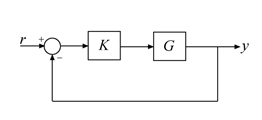
      Feedback loop formed by controller K and plant G with negative unit feedback, feedback(G*K,eye(n)).

      Stability of this loop is preserved as long as the approximation error of the reduced plant is smaller than the robustness margin for this loop given by ncfmargin(G,K).

      For controllers computed with ncfsyn (Robust Control Toolbox), reducing the controller Ks that ncfsyn computes for the shaped controller Gs is preferable. Both Ks and Gs are returned by ncfsyn in the info output argument. You can then compute Kr, the reduced controller for the original plant G, from Kr = W1KsrW2, where W1 and W2 are the shaping weights used with ncfsyn. For an example, see Reduce Controller Order While Preserving Stability and Robustness.

      For controllers obtained by other techniques, reduction with this method also preserves stability if the error does not exceed the ncfmargin margin. However, such reduction can partially remove integral action and introduce steady-state tracking errors. Therefore, removing any integrator terms from the controller before reduction and replacing them in the reduced controller is recommended.

    Algorithms

    The balanced truncation of normalized coprime factors algorithm performs these steps to reduce the input model G to the desired order k.

    1. Find the left normalized coprime factorization [Ml,Nl] of G, where G = Ml\Nl (see lncf (Robust Control Toolbox)).

    2. Obtain the kth-order approximation [Mk,Nk] of [Ml,Nl], using balanced model truncation with absolute error control (see the Algorithms section of BalancedTruncation).

    3. Set Gred = Mk\Nk.

    Version History

    Introduced in R2023b