State Estimation with Wrapped Measurements Using Extended Kalman Filter
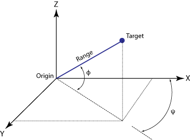
This example shows how to use the extended Kalman filter algorithm for nonlinear state estimation for 3-D tracking involving circularly wrapped angle measurements. For target tracking, sensors usually employ a spherical frame to report the position of an object in terms of azimuth, range, and elevation. The angular measurements from this set are reported within certain bounds. For instance, azimuth angles are reported within a range of to or to . However, tracking is usually done in a rectangular frame, which necessitates the use of a nonlinear filter that can handle the nonlinear transformations required to transform spherical measurements into rectangular states.
This example uses a constant velocity model to track the three-dimensional positions and velocities of a target. An Extended Kalman Filter is used as the nonlinear filter to track the states of this object. This filter uses azimuth (), range, and elevation () readings as measurements during this tracking exercise.
The constant velocity 3-D plant model for this example consists of positions and velocities in the three axes as follows:
The range, azimuth, and elevation angles are given by:
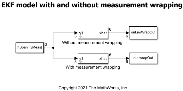
Computing the residual between the actual measurement and expected measurement is an essential step in the filtering process. Without the necessary precautions, the residual values may be large for an object located near the wrapping boundary. This causes the filter to diverge from the accurate state, leading to an inaccurate state estimate. This example demonstrates how to handle such situations by using measurement wrapping. A Simulink® model is used to demonstrate the difference in tracked states when used with and without measurement wrapping.
State Estimation - Without Measurement Wrapping
First provide your initial state guess and specify the model name.
rng(0)
initialStateGuess = [-100 0 0 0 0 0]';
modelName = 'modelEKFWrappedMeasurements';
Generate the measurements based on the noise covariance as follows:
dt = 3;
tSpan = 0:dt:100;
yTrue = zeros(length(tSpan),3);
yMeas = zeros(size(yTrue));
noiseCovariance = diag([20 0.5 0.5]);
xCurrent = initialStateGuess;

for i = 1:numel(tSpan)
   xTrue = stateTransitionFcn(xCurrent);
   yTrue(i,:) = (measurementFcn(xTrue))';
   yMeas(i,:) = yTrue(i,:) + (chol(noiseCovariance)*randn(3,1))';
   xCurrent = xTrue;
end
Simulate the model.
out = sim(modelName);
xEstNoWrap = zeros(numel(tSpan),length(initialStateGuess));
xEstWithWrap = zeros(numel(tSpan),length(initialStateGuess));
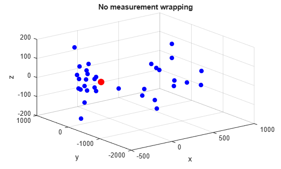
Run the filter and visualize the state convergence on a 3-D plot.
figure()
plot3(initialStateGuess(1), initialStateGuess(3), initialStateGuess(5),'ro','MarkerFaceColor','r','MarkerSize',9);
grid
hold on;

% Plot options
xlabel('x');
ylabel('y');
zlabel('z');
title('No measurement wrapping');

% Run filter
for i = 1:numel(tSpan)
   xEst = out.noWrapOut(i,:);
   plot3(xEst(1),xEst(3),xEst(5),'bo','MarkerFaceColor','b');
   hold on;
   xEstNoWrap(i,:) = xEst;
end
hold off
State Estimation - With Measurement Wrapping
Now, enable the measurement wrapping and run the filter. Visualize the state convergence on a 3-D plot.
figure()
% Run filter
for i = 1:numel(tSpan)
   xEst = out.wrapOut(i,:);
   plot3(xEst(1),xEst(3),xEst(5),'bo','MarkerFaceColor','b');
   hold on;
   xEstWithWrap(i,:) = xEst;
end
plot3(initialStateGuess(1), initialStateGuess(3), initialStateGuess(5),'ro','MarkerFaceColor','r','MarkerSize',9);
grid
title('With measurement wrapping');
hold off
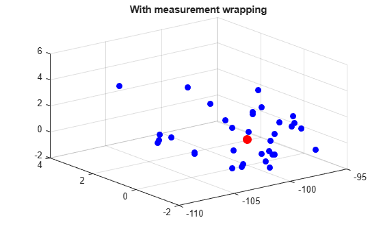
From the plot above, observe that the scale of the three axes is a lot smaller than the 3-D plot for the case without measurement wrapping. This denotes that there is better convergence when measurement wrapping is enabled.
Validation
Compare the estimation errors for both cases on the same plot.
figure()
subplot(3,1,1)
plot(xEstNoWrap(:,1) - xTrue(1));
hold on
plot(xEstWithWrap(:,1) - xTrue(1));
ylim([-500 1200])
title('e_x');
hold off

subplot(3,1,2)
plot(xEstNoWrap(:,3) - xTrue(3));
hold on
plot(xEstWithWrap(:,3) - xTrue(3));
ylim([-2000 1000])
hold off
title('e_y');

subplot(3,1,3)
plot(xEstNoWrap(:,5) - xTrue(5));
hold on
plot(xEstWithWrap(:,5) - xTrue(5));
ylim([-200 200])
hold off
title('e_z');

sgtitle('Estimation Error Plot')
legend('No Wrapping', 'With Wrapping','location','best')
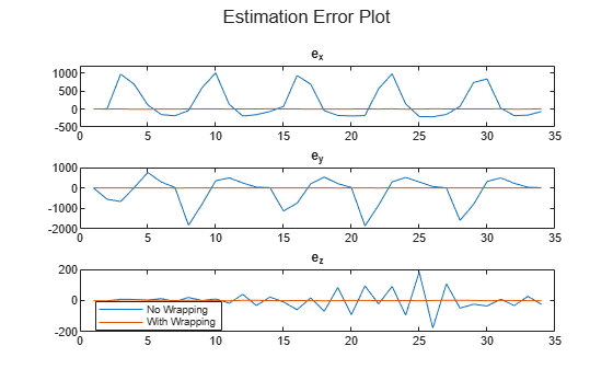
Observe that the errors are comparatively much larger in all the three axes for the case without measurement wrapping.
Summary
This example shows how to use an Extended Kalman Filter block for state estimation of a nonlinear system with and without measurement wrapping. The state estimation with wrapping enabled is observed to provide more accurate state estimates as determined by the 3-D and error plots.
Supporting Functions
State Transition Function
The Extended Kalman Filter block requires a function that describes the evolution of states from one time step to the next. This is typically called the state transition function. For this example, the contents of the state transition function contained in stateTransitionFcn.m is as follows:
function x = stateTransitionFcn(x)
   dt = 3;
   A = [1 dt 0 0  0 0;
        0 1  0 0  0 0;
        0 0  1 dt 0 0;
        0 0  0 1  0 0;
        0 0  0 0  1 dt;
        0 0  0 0  0  1];
   x = A*x;
end
Measurement Function
The Extended Kalman Filter block also needs a function that describes how the model states are related to sensor measurements. This is the measurement function. For this example, the contents of the measurement function contained in measurementFcn.m is as follows:
function [y, bounds] = measurementFcn(x)
   xPos = x(1);
   yPos = x(3);
   zPos = x(5);

   % Range
   r = sqrt(xPos^2 + yPos^2 + zPos^2);
   % Azimuth
   psi = atan2d(yPos,xPos);
   % Elevation
   phi = asind(zPos/r);
   % Combined measurement
   y = [r ; psi; phi];
   bounds = [-inf inf;-180 180; -90 90];
end