Visualize Automated Parking Valet Using Cuboid Simulation
This example shows how to visualize the motion of a vehicle as it navigates a parking lot in a cuboid driving scenario environment. It closely follows the Visualize Automated Parking Valet Using Unreal Engine Simulation example.
Visualization Workflow
Automated Driving Toolbox™ provides a cuboid driving scenario environment that enables you to rapidly author scenarios, generate detections using low-fidelity radar and camera sensors, and test controllers and tracking and sensor fusion algorithms in both MATLAB® and Simulink®. The Automated Parking Valet in Simulink example shows how to design a path planning and vehicle control algorithm for an automated parking valet system in Simulink. This example shows how to augment that algorithm to visualize vehicle motion in a scenario using a drivingScenario object. The steps in this workflow are:
Create a driving scenario containing a parking lot.
Create a
vehicleCostmapfrom the driving scenario.Create a route plan for the ego vehicle in the scenario.
Simulate the scenario in Simulink and visualize the motion of the vehicle in the driving scenario.
Create Driving Scenario
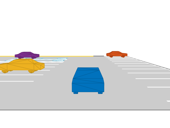
The drivingScenario object enables you to author low-fidelity scenes. Create a drivingScenario object and add the elements necessary to model a parking maneuver:
Create a parking lot that contains grids of parking spaces.
Add the ego vehicle.
Insert static vehicles at various locations on the parking lot to serve as obstacles.
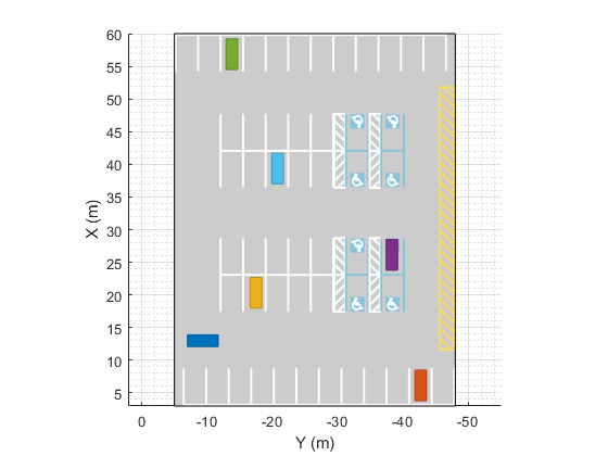
% Get a list of systems that are open now so any systems opened during this
% example can be closed at the end.
startingOpenSystems = find_system('MatchFilter', @Simulink.match.allVariants);

% Create drivingScenario object
scenario = drivingScenario;

% Create parking lot
lot = parkingLot(scenario,[3 -5; 60 -5; 60 -48; 3 -48]);

% Create parking spaces
cars = parkingSpace(Width=3.3);
accessible = parkingSpace(Type="Accessible",Width=3.3);
accessLane = parkingSpace(Type="NoParking",MarkingColor=[1 1 1],Width=1.5);
fireLane = parkingSpace(Type="NoParking",Length=2,Width=40);

% Insert parking spaces
insertParkingSpaces(lot,cars,Edge=2);
insertParkingSpaces(lot,cars,Edge=4);
insertParkingSpaces(lot,[cars accessLane accessible accessLane accessible], ...
    [5 1 1 1 1],Rows=2,Position=[42 -12]);
insertParkingSpaces(lot,[cars accessLane accessible accessLane accessible], ...
    [5 1 1 1 1],Rows=2,Position=[23 -12]);
insertParkingSpaces(lot,fireLane,1,Edge=3,Offset=8);

% Add the ego vehicle
egoVehicle = vehicle(scenario, ...
    ClassID=1, ...
    Position=[13 8 0].*[1 -1 1], ...
    Yaw=270, ...
    Mesh=driving.scenario.carMesh, ...
    Name="Ego");

% Add stationary vehicles
car1 = vehicle(scenario, ...
    ClassID=1, ...
    Position=[7.5 -42.7 0.01], ...
    Yaw=180, ...
    Mesh=driving.scenario.carMesh);

car2 = vehicle(scenario, ...
    ClassID=1, ...
    Position=[19 -17.5 0.01], ...
    Mesh=driving.scenario.carMesh);

car3 = vehicle(scenario, ...
    ClassID=1, ...
    Position=[27.5 -38.3 0.01], ...
    Yaw=180, ...
    Mesh=driving.scenario.carMesh);

car4 = vehicle(scenario, ...
    ClassID=1, ...
    Position=[55.5 -13.8 0.01], ...
    Mesh=driving.scenario.carMesh);

car5 = vehicle(scenario, ...
    ClassID=1, ...
    Position=[38 -20.8 0.01], ...
    Mesh=driving.scenario.carMesh);

% Plot drivingScenario
plot(scenario)
Create Costmap from Driving Scenario
To create a costmap from the driving scenario, follow these steps:
Capture a screenshot of the plot of the driving scenario using the
saveasCreate a spatial referencing object using the
imref2dRead the PNG image into a variable in the base workspace using the
imread
You can then display the image using imshow
% Load the image data
load("SceneImageData.mat","sceneImage","sceneRef")

% Visualize the scene image
figure
imshow(sceneImage, sceneRef);
xlabel('X (m)');
ylabel('Y (m)');
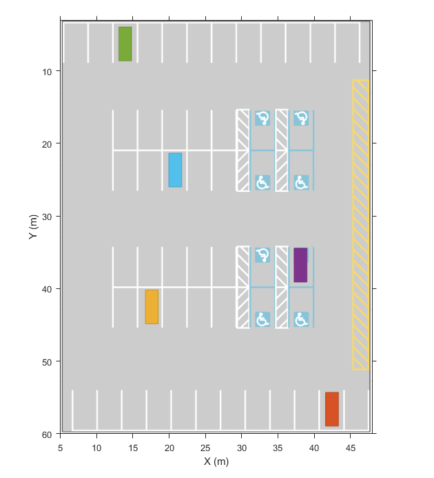
The screenshot is an accurate depiction of the environment up to some resolution. You can use this image to create a vehicleCostmap
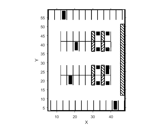
First, estimate free space by using the image. Free space is the area where a vehicle can drive without collision with static objects, such as parked cars, cones, and road boundaries, and without crossing marked lines. In this example, you can estimate the free space based on the color of the image. Use the Color Thresholder app to perform segmentation and generate a binary image from the image. You can also use the helperCreateCostmapFromImage helper function, detailed at the end of this example, to generate the binary image:
sceneImageBinary = helperCreateCostmapFromImage(sceneImage);
Next, create a costmap from the binary image. Use the binary image to specify the cost value at each cell.
% Get the left-bottom corner location of the map
mapLocation = [sceneRef.XWorldLimits(1) sceneRef.YWorldLimits(1)]; % [meters meters]

% Compute resolution
mapWidth = sceneRef.XWorldLimits(2) - sceneRef.XWorldLimits(1); % meters
cellSize = mapWidth/size(sceneImageBinary,2);

% Create the costmap
costmap = vehicleCostmap(im2single(sceneImageBinary),CellSize=cellSize,MapLocation=mapLocation);

figure
plot(costmap,Inflation='off')
legend off
You must also specify the dimensions of the vehicle that parks in the driving scenario. This example uses the vehicle dimensions described in the Create Actor and Vehicle Trajectories Programmatically example.
frontOverhang = egoVehicle.FrontOverhang;
rearOverhang = egoVehicle.RearOverhang;
vehicleWidth = egoVehicle.Width;
vehicleHeight = egoVehicle.Height;
vehicleLength = egoVehicle.Length;
centerToFront = (vehicleLength/2) - frontOverhang;
centerToRear = (vehicleLength/2) - rearOverhang;

vehicleDims = vehicleDimensions(vehicleLength,vehicleWidth,vehicleHeight, ...
    FrontOverhang=frontOverhang,RearOverhang=rearOverhang);
costmap.CollisionChecker.VehicleDimensions = vehicleDims;
Set the inflation radius by specifying the number of circles enclosing the vehicle.
costmap.CollisionChecker.NumCircles = 5;
Create Route Plan for Ego Vehicle
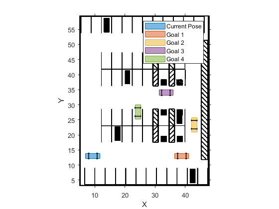
The global route plan is a sequence of lane segments that the vehicle must traverse to reach a parking spot. In this example, the route plan has been created and stored in a table. For more information on creating a route plan, review the Automated Parking Valet in Simulink example. Before simulation, the PreLoadFcn callback function of the model loads the route plan.
data = load("routePlanDrivingScenario.mat");
routePlan = data.routePlan %#ok<NOPTS>

% Plot vehicle at the starting pose
egoVehicle.Position = [routePlan.StartPose(1,2) routePlan.StartPose(1,1) 0].*[1 -1 1];
egoVehicle.Yaw = routePlan.StartPose(1,3) - 90;

startPose = routePlan.StartPose(1,:);
hold on
helperPlotVehicle(startPose,vehicleDims,DisplayName="Current Pose")
legend

for n = 1:height(routePlan)
    % Extract the goal waypoint
    vehiclePose = routePlan{n, 'EndPose'};

    % Plot the pose
    legendEntry = sprintf("Goal %i",n);
    helperPlotVehicle(vehiclePose,vehicleDims,DisplayName=legendEntry);
    hold on
end
hold off
routePlan =

  4×3 table

         StartPose                EndPose           Attributes
    ____________________    ____________________    __________

       8      13       0    37.5      13       0    1×1 struct
    37.5      13       0      43      22      90    1×1 struct
      43      22      90      35      34     180    1×1 struct
      35      34     180    24.3      29     270    1×1 struct
Explore Model
The APVWithDrivingScenario model extends the one used in the Automated Parking Valet in Simulink example by adding a plot to visualize the vehicle in a driving scenario. Open the model.
helperCloseFigures

modelName = "APVWithDrivingScenario";
open_system(modelName)
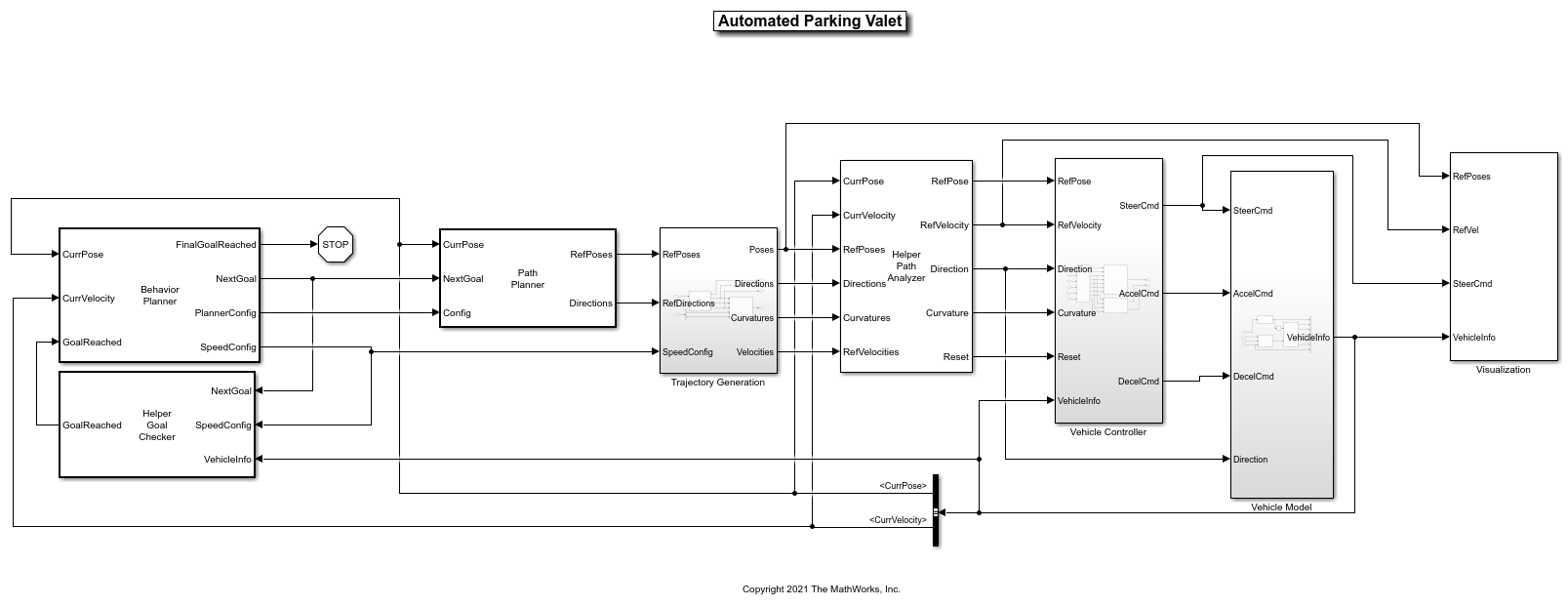
The Path Planner block of the Simulink model computes an optimal trajectory for the ego vehicle using the route plan created earlier. The model generates a pose for the ego vehicle at each time step. The model feeds this pose to the Visualization block, which updates the drivingScenario object and the costmap visualization. Plot the driving scenario from the perspective of the ego vehicle.
chasePlot(egoVehicle,ViewHeight=3,ViewPitch=5,Meshes="on");
movegui("east");
Visualize Vehicle Motion
Simulate the model to see how the vehicle drives into the desired parking spot.
sim(modelName)

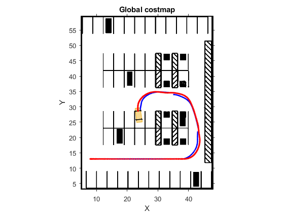
As the simulation runs, the Simulink environment updates the position and orientation of the vehicle in the driving scenario using the Visualization block. The Automated Parking Valet figure displays the planned path in blue and the actual path of the vehicle in red. The Parking Maneuver figure shows a local costmap used in searching for the final parking maneuver.
Close the model and the figures.
endingOpenSystems = find_system('MatchFilter', @Simulink.match.allVariants);
bdclose(setdiff(endingOpenSystems,startingOpenSystems))
helperCloseFigures
Supporting Functions
helperCreateCostmapFromImage
function BW = helperCreateCostmapFromImage(sceneImage)
%helperCreateCostmapFromImage Create a costmap from an RGB image.

% Call the autogenerated code from the Color Thresholder app.
BW = helperCreateMask(sceneImage);

% Smooth the image.
BW = im2uint8(medfilt2(BW));

% Resize.
BW = imresize(BW,0.5);

% Compute complement.
BW = imcomplement(BW);
end
helperCreateMask
function [BW,maskedRGBImage] = helperCreateMask(RGB)
%helperCreateMask  Threshold RGB image using auto-generated code from
%Color Thresholder app.
%  [BW,maskedRGBImage] = createMask(RGB) thresholds image RGB using
%  autogenerated code from the Color Thresholder app. The colorspace
%  and range for each channel of the colorspace have been set within the
%  app. The segmentation mask is returned in BW, and a composite of the
%  mask and original RGB image is returned in maskedRGBImage.

% Convert RGB image to chosen color space.
I = RGB;

% Define thresholds for channel 1 based on histogram settings.
channel1Min = 115.000;
channel1Max = 246.000;

% Define thresholds for channel 2 based on histogram settings.
channel2Min = 155.000;
channel2Max = 225.000;

% Define thresholds for channel 3 based on histogram settings.
channel3Min = 193.000;
channel3Max = 209.000;

% Create mask based on chosen histogram thresholds.
sliderBW = (I(:,:,1) >= channel1Min) & (I(:,:,1) <= channel1Max) & ...
    (I(:,:,2) >= channel2Min) & (I(:,:,2) <= channel2Max) & ...
    (I(:,:,3) >= channel3Min) & (I(:,:,3) <= channel3Max);
BW = sliderBW;

% Initialize output masked image based on input image.
maskedRGBImage = RGB;

% Set background pixels where BW is false to zero.
maskedRGBImage(repmat(~BW,[1 1 3])) = 0;
end
helperCloseFigures
function helperCloseFigures()
%helperCloseFigures Close all the figures except the simulation
%visualization

% Find all the figure objects
figHandles = findobj("Type","figure");

% Close the figures
for i = 1:length(figHandles)
    close(figHandles(i));
end
end
See Also
parkingLot | drivingScenario | vehicleCostmap