dsp.FrequencyDomainFIRFilter
Filter input signal in frequency domain
Description
The dsp.FrequencyDomainFIRFilter
System object™ implements frequency-domain, fast Fourier transform (FFT)-based filtering to
filter a streaming input signal. In the time domain, the filtering operation involves a
convolution between the input and the impulse response of the finite impulse response (FIR)
filter. In the frequency domain, the filtering operation involves the multiplication of the
Fourier transform of the input and the Fourier transform of the impulse response. The
frequency-domain filtering is efficient when the impulse response is very long. You can
specify the filter coefficients directly in the frequency domain by setting
NumeratorDomain to "Frequency".
This object uses the overlap-save and overlap-add methods to perform the frequency-domain
filtering. For an example showing these two methods, see Frequency Domain Filtering Using Overlap-Add and Overlap-Save. For filters with a long
impulse response length, the latency inherent to these two methods can be significant. To
mitigate this latency, the dsp.FrequencyDomainFIRFilter object partitions the
impulse response into shorter blocks and implements the overlap-save and overlap-add methods
on these shorter blocks. To partition the impulse response, set the
PartitionForReducedLatency property to true. For an
example, see Reduce Latency Through Partitioned Numerator. For more details on these
two methods and on reducing latency through impulse response partitioning, see Algorithms.
The dsp.FrequencyDomainFIRFilter
object can model single-input multiple-output (SIMO) and multiple-input multiple-output (MIMO)
systems by supporting multiple filters in the time domain and the frequency domain. For
examples, see Filter Input Signal Using 1-by-2 SIMO System and Filter Input Signal Using 3-by-2 MIMO System. You can also specify
multiple paths between each input channel and output channel pair using the
NumPaths property. For an example, see Filter Input Signal Through Multiple Propagation Paths. For more information on
modeling MIMO systems, see Modeling MIMO System with Multiple Propagation Paths. (since R2023b)
To filter the input signal in the frequency domain:
Create the
dsp.FrequencyDomainFIRFilterobject and set its properties.Call the object with arguments, as if it were a function.
To learn more about how System objects work, see What Are System Objects?
Creation
Syntax
Description
fdf = dsp.FrequencyDomainFIRFilter
fdf = dsp.FrequencyDomainFIRFilter(num)Numerator
property set to num.
Example: dsp.FrequencyDomainFIRFilter(fir1(400,2*2000/8000))
fdf = dsp.FrequencyDomainFIRFilter(PropertyName=Value)
Example: dsp.FrequencyDomainFIRFilter(Method="Overlap-add")
Properties
Unless otherwise indicated, properties are nontunable, which means you cannot change their
values after calling the object. Objects lock when you call them, and the
release function unlocks them.
If a property is tunable, you can change its value at any time.
For more information on changing property values, see System Design in MATLAB Using System Objects.
Frequency-domain filter method, specified as either
"Overlap-save" or "Overlap-add". For more
details on these two methods, see Algorithms.
Domain of the filter coefficients, specified as one of the following:
"Time"–– Specify the time-domain filter numerator in theNumeratorproperty."Frequency"–– Specify the filter's frequency response in theFrequencyResponseproperty.
FIR filter coefficients, specified as a row vector (single filter) or a matrix (multiple filters) (since R2023b) of size
F-by-NumLen, where F is the
number of filters and NumLen is the filter length. If
F is greater than 1, then its value must be a multiple of the
product of the number of input channels (columns) T and the number of
paths P you specify through the NumPaths
property. The multiplication factor determines the number of output channels
R and equals F/(T ×
P).
The coefficient values can change during simulation but the size of the numerator must remain constant.
Tunable: Yes
Dependencies
To enable this property, set NumeratorDomain to
"Time".
Data Types: single | double | int8 | int16 | int32 | int64 | uint8 | uint16 | uint32 | uint64
Complex Number Support: Yes
Frequency response of the filter, specified as a row vector, matrix, or a 3-D array (since R2024a).
When you set PartitionForReducedLatency to
true, FrequencyResponse must be a matrix of
size 2PL-by-N to represent a single filter or a
3-D array of size 2PL-by-N-by-F
to represent multiple filters (since R2024a), where
PL is the partition size, N is the number of
partitions, and F is the number of filters.
When you set
PartitionForReducedLatency to false,
FrequencyResponse can be a row vector or a matrix of size
F-by-FFTLength. If F is
greater than 1 (multiple filters), then its value must be a multiple of the product of
the number of input channels (columns) T and the number of paths
P you specify through the NumPaths property.
The multiplication factor determines the number of output channels R
and equals F/(T × P). (since R2023b)
Tunable: Yes
Dependencies
To enable this property, set NumeratorDomain to
"Frequency".
Data Types: single | double | int8 | int16 | int32 | int64 | uint8 | uint16 | uint32 | uint64
Complex Number Support: Yes
Time-domain numerator length, specified as a positive integer.
Dependencies
To enable this property, set NumeratorDomain to
"Frequency" and PartitionForReducedLatency
to false.
Data Types: single | double | int8 | int16 | int32 | int64 | uint8 | uint16 | uint32 | uint64
Flag to specify if the filter coefficients are all real, specified as
true or false.
Dependencies
To enable this property, set NumeratorDomain to
"Frequency".
Flag to partition numerator to reduce latency, specified as:
false–– The filter uses the traditional overlap-save or overlap-add method. The latency in this case isFFTLength– length(Numerator) + 1.true–– In this mode, the object partitions the numerator into segments of length specified by thePartitionLengthproperty. The filter performs overlap-save or overlap-add on each partition, and combines the partial results to form the overall output. The latency is now reduced to the partition length.
FFT length, specified as a positive integer. The default value of this property,
[], indicates that the FFT length is equal to twice the numerator
length. The FFT length must be greater than or equal to the numerator length.
Dependencies
To enable this property, set NumeratorDomain property to
"Time" and PartitionForReducedLatency
property to false.
Data Types: single | double | int8 | int16 | int32 | int64 | uint8 | uint16 | uint32 | uint64
Numerator partition length PL, specified as a positive integer less than or equal to the length of the numerator.
Dependencies
To enable this property, set the NumeratorDomain property to
"Time" and PartitionForReducedLatency
property to true.
Data Types: single | double | int8 | int16 | int32 | int64 | uint8 | uint16 | uint32 | uint64
This property is read-only.
Filter latency in samples, returned as an integer greater than 0. When
PartitionForReducedLatency is:
false–– The latency is equal toFFTLength– length(Numerator) + 1.true–– The latency is equal to the partition length.
Data Types: uint32
Since R2023b
Number of propagation paths P between each input channel and
output channel pair, specified as a positive integer. Each path is represented by a
unique filter. When you specify the number of paths to be greater than
1, the filter models multipath propagation. The filtered output
contributions from all paths between each input channel and output channel pair are
summed up.
For an example, see Filter Input Signal Through Multiple Propagation Paths.
Dependencies
To enable this property, the number of filters F must be greater than 1.
Data Types: single | double
Since R2023b
Option to sum filtered output contributions from all input channels, specified as:
true–– The object adds the filtered output from each input channel to generate an L-by-R output matrix, where L is the input frame size (number of input rows) and R is the output channels. R equals F/(T x P), where F is the number of filters, T is the number of input channels, and P is the value that you specify in theNumPathsproperty.false–– The object does not sum filtered output contributions from all input channels. The output is an L-by-R-by-T array.
For more information on how the object computes the output based on the value of the
SumFilteredOutputs property, see Modeling MIMO System with Multiple Propagation Paths.
Dependencies
To enable this property, the number of filters F must be greater than 1.
Data Types: logical
Usage
Syntax
Description
Input Arguments
Data input, specified as a matrix of size L-by-T. This object supports variable-size input signals, that is, you can change the input frame size (number of rows) even after calling the algorithm. However, the number of channels (columns) must remain constant.
Data Types: single | double
Complex Number Support: Yes
Output Arguments
Filtered output, returned as a vector, matrix, or a 3-D array.
When the number of filters
F is greater than 1 and you set
SumFilteredOutputs to:
true–– The object adds the filtered output from each input channel to generate an L-by-R output matrix, where L is the input frame size (number of input rows) and R is the number of output channels. R equals F/(T x P), where F is the number of filters, T is the number of input channels, and P is the value that you specify in theNumPathsproperty.false–– The object does not sum filtered output contributions from all input channels. The output is an L-by-R-by-T array.output(:,j,k)refers to the output from the kth input channel for the jth output channel. For example,output(:,3,2)indicates output on the third output channel from the second input channel.
(since R2023b)
For more information on how the object computes the output, see Algorithms.
The output has the same data type and complexity as the input signal.
Data Types: single | double
Complex Number Support: Yes
Object Functions
To use an object function, specify the
System object as the first input argument. For
example, to release system resources of a System object named obj, use
this syntax:
release(obj)
Examples
Filter input signal using overlap-add and overlap-save methods, and compare the outputs to the output of a time-domain FIR filter.
Initialization
Design the FIR lowpass filter coefficients using the designLowpassFIR function. The sampling frequency is 8 kHz. Specify a filter order of 400 and a cutoff frequency of 2 kHz. The impulse response has a length of 401.
order   = 400;
Fs      = 8000;
Fcutoff = 2000;
imp     = designLowpassFIR(FilterOrder=order,CutoffFrequency=2*Fcutoff/Fs);
Create two dsp.FrequencyDomainFIRFilter objects and a dsp.FIRFilter object. Set the numerator of all the three filters to imp. Delay the FIR output by the latency of the frequency-domain filter.
fdfOA = dsp.FrequencyDomainFIRFilter(imp,Method="Overlap-add");
fdfOS = dsp.FrequencyDomainFIRFilter(imp,Method="Overlap-save");
fir = dsp.FIRFilter(Numerator=imp);
dly = dsp.Delay(Length=fdfOA.Latency);
Create two dsp.SineWave objects. The sine waves have a sample rate of 8000 Hz, frame size of 256, and frequencies of 100 Hz and 3 kHz, respectively. Create a timescope object to view the filtered outputs.
frameLen  = 256;
sin_100Hz = dsp.SineWave(Frequency=100,SampleRate=Fs,...
    SamplesPerFrame=frameLen);
sin_3KHz  = dsp.SineWave(Frequency=3e3,SampleRate=Fs,...
    SamplesPerFrame=frameLen);
ts = timescope(TimeSpanSource="property",TimeSpan=5*frameLen/Fs,...
    YLimits=[-1.1 1.1],...
    ShowLegend=true,...
    SampleRate=Fs,...
    ChannelNames={"Overlap-add","Overlap-save","Direct-form FIR"});
Streaming
Stream 1e4 frames of noisy input data. Pass this data through the frequency domain filters and the time-domain FIR filter. View the filtered outputs in the time scope.
numFrames = 1e4;
for idx = 1:numFrames
    x = sin_100Hz() + sin_3KHz() + 0.01*randn(frameLen,1);
    yOA = fdfOA(x);
    yOS = fdfOS(x);
    yFIR = fir(dly(x));
    ts([yOA,yOS,yFIR]);
end

The outputs of all the three filters match exactly.
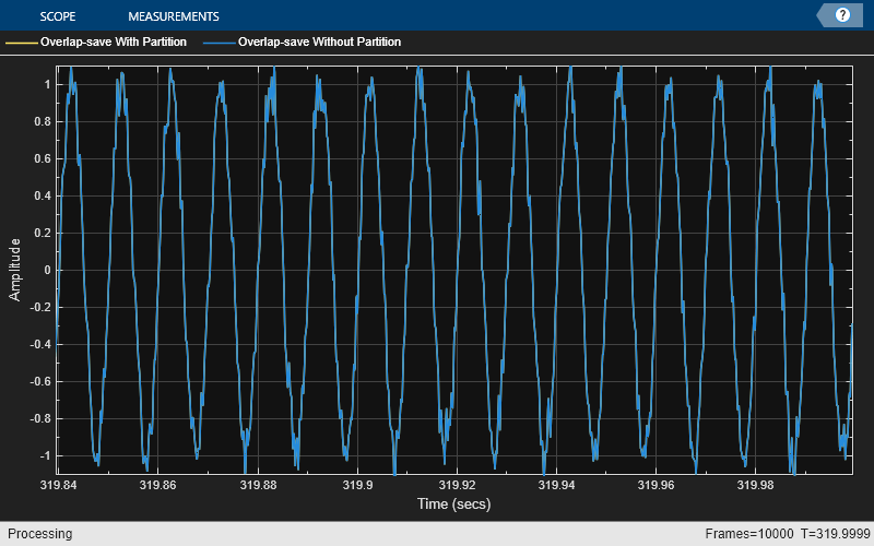
Partition the impulse response length of a frequency domain FIR filter. Compare the outputs of the partitioned filter and the original filter.
Design the FIR lowpass filter coefficients using the designLowpassFIR function. The sampling frequency is 8 kHz. Specify a filter order of 4000 and a cutoff frequency of 2 kHz. The impulse response is of length 4001.
order   = 4000;
Fs      = 8000;
Fcutoff = 2000;
imp     = designLowpassFIR(FilterOrder=order,CutoffFrequency=2*Fcutoff/Fs);
Create a dsp.FrequencyDomainFIRFilter with coefficients set to the imp vector. The latency of this filter is given by  , which is equal to 4002. By default, FFT length is equal to twice the numerator length. This makes the latency proportional to the impulse response length.
fdfOS  = dsp.FrequencyDomainFIRFilter(imp,Method="Overlap-save");
fprintf('Frequency domain filter latency is %d samples\n',fdfOS.Latency);
Frequency domain filter latency is 4002 samples
Partition the impulse response to blocks of length 256. The latency after partitioning is proportional to the block length.
fdfRL  = dsp.FrequencyDomainFIRFilter(imp,Method="Overlap-save",...
    PartitionForReducedLatency=true,...
    PartitionLength=256);
fprintf('Frequency domain filter latency is %d samples\n',fdfRL.Latency);
Frequency domain filter latency is 256 samples
Compare the outputs of the two frequency domain filters. The latency of fdfOS is 4002, and the latency of fdfRL is 256. To compare the two outputs, delay the input to fdfRL by 4002 - 256 samples.
dly = dsp.Delay(Length=(fdfOS.Latency-fdfRL.Latency));
Create two dsp.SineWave objects. The sine waves have a sample rate of 8000 Hz, frame size of 256, and frequencies of 100 Hz and 3 kHz, respectively. Create a timescope object to view the filtered outputs.
frameLen  = 256;
sin_100Hz = dsp.SineWave(Frequency=100,SampleRate=Fs,...
    SamplesPerFrame=frameLen);
sin_3KHz  = dsp.SineWave(Frequency=3e3,SampleRate=Fs,...
    SamplesPerFrame=frameLen);
ts = timescope(TimeSpanSource="property",TimeSpan=5*frameLen/Fs,...
    YLimits=[-1.1 1.1],...
    ShowLegend=true,...
    SampleRate=Fs,...
    ChannelNames={'Overlap-save With Partition','Overlap-save Without Partition'});
Stream 1e4 frames of noisy input data. Pass this data through the two frequency domain filters. View the filtered outputs in the time scope. The outputs match exactly.
numFrames = 1e4;
for idx = 1:numFrames
    x = sin_100Hz() + sin_3KHz() + .1 * randn(frameLen,1);
    yRL = fdfRL(dly(x));
    yOS = fdfOS(x);
    ts([yRL,yOS]);
end
Specify the numerator coefficients of the frequency-domain FIR filter in the frequency domain. Filter the input signal using the overlap-add method. Compare the frequency-domain FIR filter output to the corresponding time-domain FIR filter output.
Initialization
Design the FIR lowpass filter coefficients using the designLowpassFIR function. The sampling frequency is 8 kHz, and the cutoff frequency of the filter is 2 kHz. The time-domain impulse response has a length of 401. Compute the FFT of this impulse response and specify this response as the frequency response of the frequency-domain FIR filter. Set the time-domain numerator length, specified by the NumeratorLength property, to the number of elements in the time-domain impulse response.
order   = 400;
Fs      = 8000;
Fcutoff = 2000;
imp     = designLowpassFIR(FilterOrder=order,CutoffFrequency=2*Fcutoff/Fs);
H   = fft(imp,2*numel(imp));
oa  = dsp.FrequencyDomainFIRFilter(NumeratorDomain="Frequency",...
    FrequencyResponse=H,...
    NumeratorLength=numel(imp),...
    Method='Overlap-add');
fprintf('Frequency domain filter latency is %d samples\n',oa.Latency);
Frequency domain filter latency is 402 samples
Create a dsp.FIRFilter System object and specify the numerator as the time-domain coefficients computed using the designLowpassFIR function, imp. Delay the FIR output by the latency of the frequency-domain FIR filter.
fir = dsp.FIRFilter(Numerator=imp);
dly = dsp.Delay(Length=oa.Latency);
Create two dsp.SineWave objects. The sine waves generated have a sample rate of 8000 Hz, frame size of 256, and frequencies of 100 Hz and 3 kHz, respectively. Create a timescope object to view the filtered outputs.
frameLen  = 256;

sin_100Hz = dsp.SineWave(Frequency=100,SampleRate=Fs,...
    SamplesPerFrame=frameLen);
sin_3KHz  = dsp.SineWave(Frequency=3e3,SampleRate=Fs,...
    SamplesPerFrame=frameLen);

ts = timescope(YLimits=[-1.1 1.1],...
    TimeSpanSource="property",TimeSpan=5*frameLen/Fs,...
    ShowLegend=true,...
    SampleRate=Fs,...
    ChannelNames={'Overlap-add','Direct-form FIR'});
Streaming
Stream 1e4 frames of noisy input data. Pass this data through the frequency-domain FIR filter and the time-domain FIR filter. View the filtered outputs in the time scope. The outputs of both the filters match exactly.
numFrames = 1e4;
for idx = 1:numFrames
    x = sin_100Hz() + sin_3KHz() + 0.01 * randn(frameLen,1);
    y1 = oa(x);
    y2 = fir(dly(x));
    ts([y1,y2]);
end

Since R2024a
Filter an input signal using a 1-by-2 SIMO system with two distinct paths between the input and each output. Partition the filters to reduce latency.
Design four lowpass FIR filters, each with a different cutoff frequency, specified in normalized frequency units. The filter order for each filter is 4000 and the sampling rate is 8000 Hz. The SIMO system models one input channel, two output channels, and two paths between each input channel-output channel pair.
order = 4000;
Fs   = 8000;
num  = [ % Path 1, Output Channel 1
    designLowpassFIR(FilterOrder=order,CutoffFrequency=0.2);...
    % Path 2, Output Channel 1
    designLowpassFIR(FilterOrder=order,CutoffFrequency=0.3);...
    % Path 1, Output Channel 2
    designLowpassFIR(FilterOrder=order,CutoffFrequency=0.4);...
    % Path 2, Output Channel 2
    designLowpassFIR(FilterOrder=order,CutoffFrequency=0.5)];
Initialize the dsp.FrequencyDomainFIRFilter object with the array of filters. Set the partition length to 256 and the number of paths to 2. The object uses the Overlap-save method by default.
obj = dsp.FrequencyDomainFIRFilter(Numerator=num,...
    PartitionForReducedLatency=true, PartitionLength=256, NumPaths=2)
obj =
dsp.FrequencyDomainFIRFilter with properties:
Method: 'Overlap-save'
NumeratorDomain: 'Time'
Numerator: [4×4001 double]
NumPaths: 2
SumFilteredOutputs: true
PartitionForReducedLatency: true
PartitionLength: 256
Latency: 256
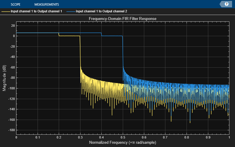
Visualize the frequency response of the individual filters.
visualize(obj)

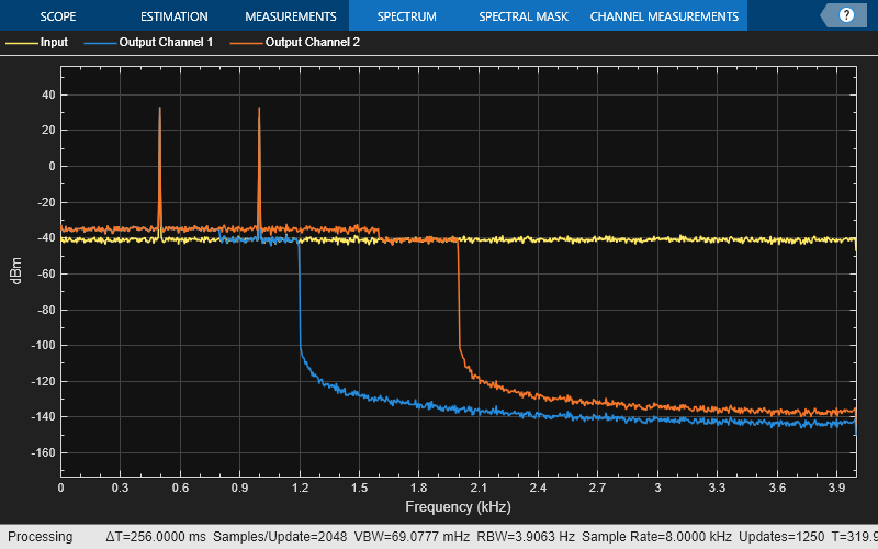
The input contains two sinusoidal signals, each with a frame length of 256. The first sinusoidal signal has a frequency of 500 Hz (or 0.125 in normalized frequency units) and the second sinusoidal signal has a frequency of 1000 Hz (or 0.25 in normalized frequency units).
frameLen  = 256;
sin_500Hz = dsp.SineWave(Frequency=500,SampleRate=Fs,...
    SamplesPerFrame=frameLen);
sin_1KHz  = dsp.SineWave(Frequency=1e3,SampleRate=Fs,...
    SamplesPerFrame=frameLen);
Initialize a spectrumAnalyzer object to view the spectrum of the input and the filtered output.
specScope = spectrumAnalyzer(SampleRate=Fs,PlotAsTwoSidedSpectrum=false,...
    ChannelNames={'Input','Output Channel 1',...
    'Output Channel 2'},...
    ShowLegend=true);
Stream in 1e4 frames of the noisy input sinusoidal signal. The input noise is white Gaussian with a mean of 0 and a variance of 0.01. Pass the signal through the designed filter. Visualize the spectrum of the input and output signals in the spectrum analyzer.
for idx = 1:1e4
    x = sin_500Hz() + sin_1KHz() + 0.01 * randn(frameLen, 1);
    y = obj(x);
    specScope([x, y]);
end
Visualize the frequency response of the sum of all filter paths between each input channel and output channel by setting SumFilterPaths to true.
visualize(obj,SumFilterPaths=true)
Since R2023b
Design six lowpass FIR filters with varying cutoff frequencies. The filter order for each filter is 400 and the sampling rate is 8000 Hz. The system models three input channels, two output channels, and one path between each input channel-output channel pair.
order = 400;
Fs = 8000;
num = [% Input Channel 1, Output Channel 1
    designLowpassFIR(FilterOrder=order,CutoffFrequency=0.1);...
    % Input Channel 1, Output Channel 2
    designLowpassFIR(FilterOrder=order,CutoffFrequency=0.15);...
    % Input Channel 2, Output Channel 1
    designLowpassFIR(FilterOrder=order,CutoffFrequency=0.2);...
    % Input Channel 2, Output Channel 2
    designLowpassFIR(FilterOrder=order,CutoffFrequency=0.25);...
    % Input Channel 3, Output Channel 1
    designLowpassFIR(FilterOrder=order,CutoffFrequency=0.3);...
    % Input Channel 3, Output Channel 2
    designLowpassFIR(FilterOrder=order,CutoffFrequency=0.35)];
Initialize the dsp.FrequencyDomainFIRFilter object with the array of filters. Specify the filtering method as "Overlap-save". The SumFilteredOutputs property is true by default.
 filt = dsp.FrequencyDomainFIRFilter(Numerator=num,...
    Method='Overlap-save')
filt =
  dsp.FrequencyDomainFIRFilter with properties:

                        Method: 'Overlap-save'
               NumeratorDomain: 'Time'
                     Numerator: [6×401 double]
                      NumPaths: 1
            SumFilteredOutputs: true
    PartitionForReducedLatency: false
                     FFTLength: []
                       Latency: 402
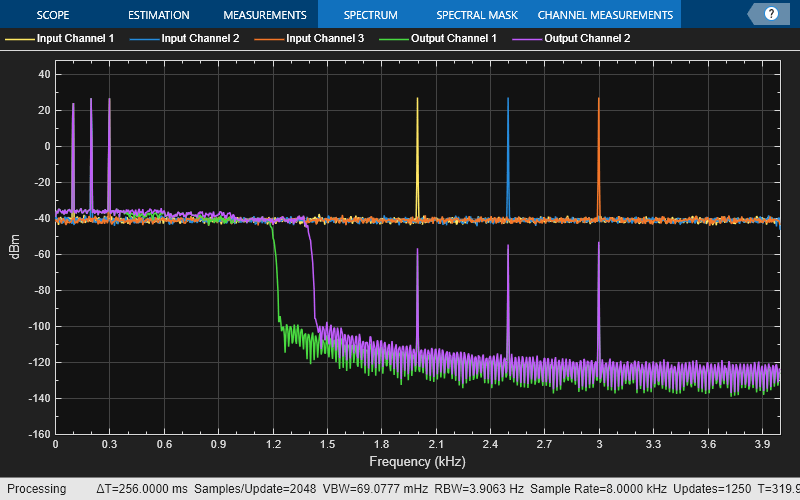
The input contains two sinusoidal signals each with a frame length of 256. The first sinusoidal signal contains tones at 100 Hz, 200 Hz, and at 300 Hz. The second sinusoidal signal contains tones at 2 kHz, 2.5 kHz, and at 3 kHz.
 frameLen = 256;
 sin_Hz = dsp.SineWave(Frequency=[100 200 300],SampleRate=Fs,...
     SamplesPerFrame=frameLen);
 sin_KHz = dsp.SineWave(Frequency=[2e3 2.5e3 3e3],SampleRate=Fs,...
     SamplesPerFrame=frameLen);
Initialize a spectrumAnalyzer object to view the spectrum of the input and the filtered output.
 specScope = spectrumAnalyzer(SampleRate=Fs,PlotAsTwoSidedSpectrum=false, ...
     ChannelNames={'Input Channel 1','Input Channel 2','Input Channel 3', ...
     'Output Channel 1','Output Channel 2'},ShowLegend=true);
Stream in 1e4 frames of the noisy input sinusoidal signal. The input noise is white Gaussian with a mean of 0 and a variance of 0.01. Pass the signal through the designed filter. Visualize the spectrum of the input and output signals in spectrum analyzer.
  for idx = 1:1e4
     x = sin_Hz()+sin_KHz()+0.01*randn(frameLen,3);
     y = filt(x);
     specScope([x,y]);
 end
Since R2023b
Filter an input signal through three distinct paths between the input and the output by specifying three filters to model the frequency responses across each path.
Design multiple lowpass FIR filters with varying fractional delays. The filter order for each filter is 400 and the sampling rate is 8000 Hz.
order = 400;
Fs = 8000;
num = [designFracDelayFIR(0.1,order); % Path 1
    designFracDelayFIR(0.2,order); % Path 2
    designFracDelayFIR(0.3,order); % Path 3
    ];
Initialize the dsp.FrequencyDomainFIRFilter object with the array of filters. Set the filtering method to "Overlap-add" and the number of propagation paths to 3. The object models a single-input single-output (SISO) system. The SumFilteredOutputs property is true by default.
filt = dsp.FrequencyDomainFIRFilter(Numerator=num, ...
    Method='overlap-add',NumPaths=3)
filt =
  dsp.FrequencyDomainFIRFilter with properties:

                        Method: 'Overlap-add'
               NumeratorDomain: 'Time'
                     Numerator: [3×400 double]
                      NumPaths: 3
            SumFilteredOutputs: true
    PartitionForReducedLatency: false
                     FFTLength: []
                       Latency: 401
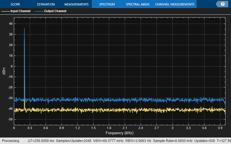
The input contains two sinusoidal signals each with a frame length of 1024. The first sinusoidal signal contains a tone at 200 Hz. The second sinusoidal signal contains a tone at 4 kHz.
frameLen = 1024;
sin_200Hz = dsp.SineWave(Frequency=200,SampleRate=Fs, ...
    SamplesPerFrame=frameLen);
sin_4KHz = dsp.SineWave(Frequency=4e3,SampleRate=Fs, ...
    SamplesPerFrame=frameLen);
Initialize a spectrumAnalyzer object to view the spectrum of the input and the filtered output.
specScope = spectrumAnalyzer(SampleRate=Fs,PlotAsTwoSidedSpectrum=false, ...
    ChannelNames={'Input Channel','Output Channel'},ShowLegend=true);
Stream in 1e3 frames of the noisy input sinusoidal signal. The input noise is white Gaussian with a mean of 0 and a variance of 0.01. Pass the signal through the designed filter. Visualize the spectrum of the input and output signals in spectrum analyzer.
for idx = 1:1e3
    x = sin_200Hz()+sin_4KHz()+0.01*randn(frameLen,1);
    y = filt(x);
    specScope([x,y])
end
Algorithms
Overlap-save and overlap-add are the two frequency-domain FFT-based filtering methods this algorithm uses.
The overlap-save method is implemented using the following approach:

The input stream is partitioned into overlapping blocks of size FFTLen, with an overlap factor of NumLen – 1 samples. FFTLen is the FFT length and NumLen is the length of the FIR filter numerator. The FFT of each block of input samples is computed and multiplied with the length-FFTLen FFT of the FIR numerator. The inverse fast Fourier transform (IFFT) of the result is performed, and the last FFTLen – NumLen + 1 samples are saved. The remaining samples are dropped.
The latency of overlap-save is FFTLen – NumLen + 1. The first FFTLen – NumLen + 1 samples are equal to zero. The filtered value of the first input sample appears as the FFTLen – NumLen + 2 output sample.
Note that the FFT length must be larger than the numerator length, and is typically set to a value much greater than NumLen.
The overlap-add method is implemented using the following approach:

The input stream is partitioned into blocks of length FFLen – NumLen + 1, with no overlap between consecutive blocks. Similar to overlap-save, the FFT of the block is computed, and multiplied by the FFT of the FIR numerator. The IFFT of the result is then computed. The first NumLen + 1 samples are modified by adding the values of the last NumLen + 1 samples from the previous computed IFFT.
The latency of overlap-add is FFTLen – NumLen + 1. The first FFTLen – NumLen + 1 samples are equal to zero. The filtered value of the first input sample appears as the FFTLen – NumLen + 2 output sample.
With an FFT length that is twice the length of the FIR numerator, the latency roughly equals the length of the FIR numerator. If the impulse response is very long, the latency becomes significantly large. However, frequency domain FIR filtering is still faster than the time-domain filtering. To mitigate the latency and make the frequency domain filtering even more efficient, the algorithm partitions the impulse response into multiple short blocks and performs overlap-save or overlap-add on each block. The results of the different blocks are then combined to obtain the final output. The latency of this approach is of the order of the block length, rather than the entire impulse response length. This reduced latency comes at the cost of additional computation. For more details, see [1].
These diagrams present a generalized representation of a frequency-domain FIR filter using multiple filters to process signals between multiple input channels and output channels. This diagram models multiple paths between each input channel-output channel pair.
SumFilteredOutputs is
true
The algorithm passes the first input channel through the first set of R × P filters within which ((i − 1) × P + 1) to (i × P) filters compute the output for the ith output channel. The algorithm passes the second input channel through the next set of R × P filters, and the sequence continues until the last input channel passes through the filter F.
The algorithm adds the filtered output contributions from all input channels before sending them as the respective output channel.
The input signal is of size L-by-T.
L is the input frame size (number of input rows).
T is the number of input channels.
F is the number of filters. This value is the number of rows in the filter coefficients matrix.
Filter coefficients is a matrix of size F-by-numLen. Each row corresponds to a filter of length numLen.
P is the number of propagation paths between each input channel and output channel.
R is the number of output channels and equals F/(T x P).
Output signal is of size L-by-R. Each output channel is of size L-by-1.
SumFilteredOutputs is
false
The algorithm concatenates the filtered outputs and does not sum across input
channels. The output is an
L-by-R-by-T array that you
can further process before sending it to the output. For example, if you add elements in
the L-by-R-by-T array across
the third dimension, the resultant L-by-R array is
same as the output signal you get when you set SumFilteredOutputs
to true.
References
[1] Stockham, T. G., Jr. "High Speed Convolution and Correlation." Proceedings of the 1966 Spring Joint Computer Conference, AFIPS, Vol 28, 1966, pp. 229–233.
Extended Capabilities
Usage notes and limitations:
See System Objects in MATLAB Code Generation (MATLAB Coder).
Version History
Introduced in R2017bUse the new visualize function
to view the frequency response of the dsp.FrequencyDomainFIRFilter
object.
Starting R2024a, you can set PartitionForReducedLatency to
true when you specify multiple filters. Setting
PartitionForReducedLatency to true enables
partitioning on the filters to reduce latency.
You can model MIMO systems by specifying multiple filters in the time and frequency domains. You can also specify multiple paths between each input and output pair.
MATLAB Command
You clicked a link that corresponds to this MATLAB command:
Run the command by entering it in the MATLAB Command Window. Web browsers do not support MATLAB commands.
Seleziona un sito web
Seleziona un sito web per visualizzare contenuto tradotto dove disponibile e vedere eventi e offerte locali. In base alla tua area geografica, ti consigliamo di selezionare: .
Puoi anche selezionare un sito web dal seguente elenco:
Come ottenere le migliori prestazioni del sito
Per ottenere le migliori prestazioni del sito, seleziona il sito cinese (in cinese o in inglese). I siti MathWorks per gli altri paesi non sono ottimizzati per essere visitati dalla tua area geografica.
Americhe
- América Latina (Español)
- Canada (English)
- United States (English)
Europa
- Belgium (English)
- Denmark (English)
- Deutschland (Deutsch)
- España (Español)
- Finland (English)
- France (Français)
- Ireland (English)
- Italia (Italiano)
- Luxembourg (English)
- Netherlands (English)
- Norway (English)
- Österreich (Deutsch)
- Portugal (English)
- Sweden (English)
- Switzerland
- United Kingdom (English)