printToFigure
Description
printToFigure( prints the display window
of the scope)scope object to a new MATLAB® figure. The figure is visible by default.
Examples
Use the printToFigure function to print the spectrumAnalyzer object display window to a new MATLAB® figure.
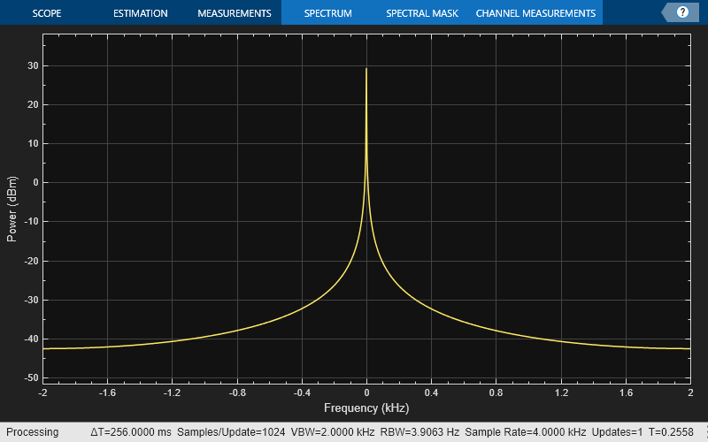
Generate a chirp signal and use the spectrumAnalyzer object to display the spectrum of the chirp. This plot shows the default color and style settings of the spectrumAnalyzer object.
chirp = dsp.Chirp(SweepDirection="Bidirectional", ...
    TargetFrequency=2000, ...
    InitialFrequency=0,...
    TargetTime=400, ...
    SweepTime=400, ...
    SamplesPerFrame=1024, ...
    SampleRate=4000);
scope = spectrumAnalyzer(AveragingMethod="exponential",...
    ForgettingFactor=0,SampleRate=4000);
scope(chirp());
Change the background color and the axes color of the plot to "white". Set the font color and line color to "black".
scope.BackgroundColor = "white";
scope.AxesColor = "white";
scope.FontColor = "black";
scope.LineColor = "black";
show(scope)
release(scope)
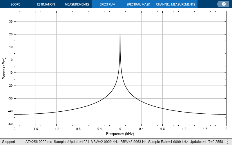
Print the display of the chirp spectrum to a new MATLAB figure. The function returns a handle to the figure.
scopeFig = printToFigure(scope);

The handle to the figure scopeFig lets you modify the appearance and the behavior of the figure window.
Specify a figure name and change the size of the figure to 400-by-250 pixels.
scopeFig.Name="Spectrum of Chirp Signal";
scopeFig.NumberTitle="off";
scopeFig.Position=[1 1 400 250];
When printing to figure, you can make the figure invisible by setting the Visible argument to false.
scopeFig = printToFigure(scope,Visible=false);
Use the printToFigure function to print the dsp.ArrayPlot object display window to a new MATLAB® figure.
Create a dsp.ArrayPlot object.
scope=dsp.ArrayPlot;
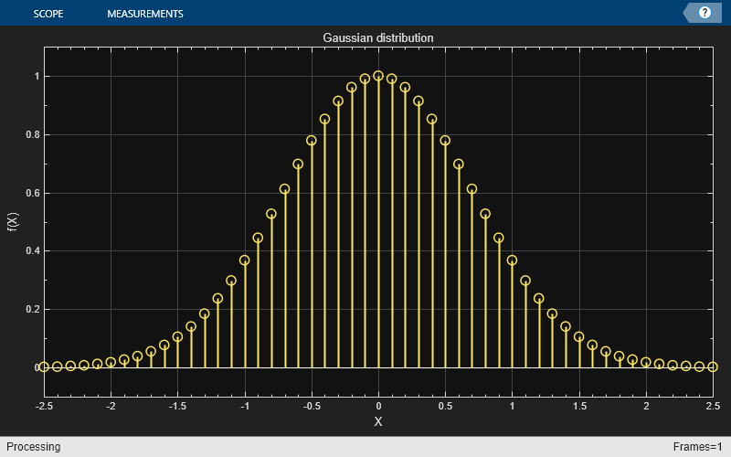
Set ArrayPlot properties to display a Gaussian distribution.
scope.YLimits = [-0.1 1.1];
scope.XOffset = -2.5;
scope.SampleIncrement = 0.1;
scope.Title = "Gaussian distribution";
scope.XLabel = "X";
scope.YLabel = "f(X)";
Plot the Gaussian distribution.
scope(exp(-(-2.5:.1:2.5) .* (-2.5:.1:2.5))');
Change the background color and the axes color of the plot to "white". Set the font color to "black" and the line color to "blue".
scope.BackgroundColor = "white";
scope.AxesColor = "white";
scope.FontColor = "black";
scope.LineColor = "blue";
show(scope)
release(scope)
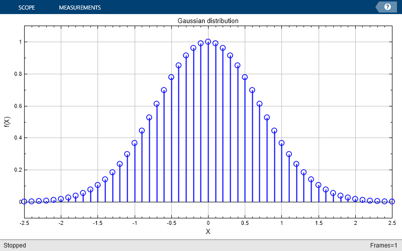
Print the display of the Gaussian distribution to a new MATLAB figure. The function returns a handle to the figure.
scopeFig = printToFigure(scope);

The handle to the figure scopeFig lets you modify the appearance and the behavior of the figure window.
Specify a figure name and change the size of the figure to 400-by-250 pixels.
scopeFig.Name="Gaussian Distribution";
scopeFig.NumberTitle="off";
scopeFig.Position=[1 1 400 250];
When printing to figure, you can make the figure invisible by setting the Visible argument to false.
scopeFig = printToFigure(scope,Visible=false);
Use the printToFigure function to print the timescope object display window to a new MATLAB® figure.
The timescope object requires one of these products:
DSP System Toolbox™
Navigation Toolbox™
Sensor Fusion and Tracking Toolbox™
View a sine wave on the time scope. This plot shows the default color and style settings of the timescope object.
f = 100;
fs = 1000;
swv = sin(2.*pi.*f.*(0:1/fs:1-1/fs)).';
scope = timescope(SampleRate=fs,...
    TimeSpanSource="property", ...
    TimeSpan=1);
scope(swv);
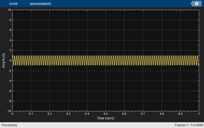
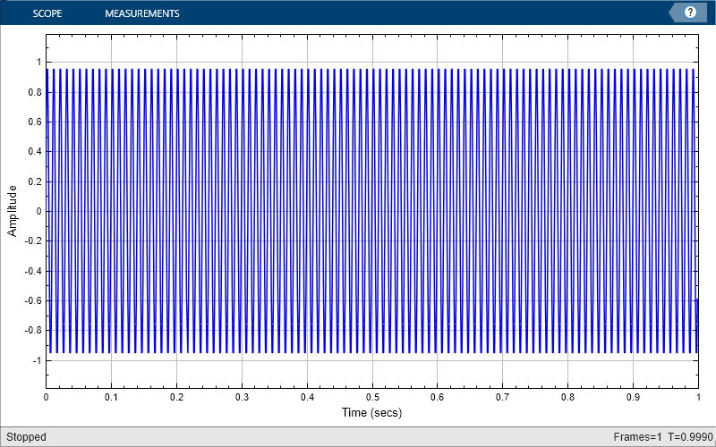
Change the background color and the axes color of the plot to "white". Set the font color to "black" and the line color to "blue".
scope.BackgroundColor = "white";
scope.AxesColor = "white";
scope.FontColor = "black";
scope.LineColor = "blue";
show(scope)
release(scope)

Print the display of the sine wave to a new MATLAB figure. The function returns a handle to the figure.
scopeFig = printToFigure(scope);
The handle to the figure scopeFig lets you modify the appearance and the behavior of the figure window.
Specify a figure name and change the size of the figure to 400-by-250 pixels.
scopeFig.Name="Sine Wave Signal";
scopeFig.NumberTitle="off";
scopeFig.Position=[1 1 400 250];
When printing to figure, you can make the figure invisible by setting the Visible argument to false.
scopeFig = printToFigure(scope,Visible=false);
Use the printToFigure function to print the dsp.DynamicFilterVisualizer object display window to a new MATLAB® figure.
Create a dsp.DynamicFilterVisualizer object.
dfv = dsp.DynamicFilterVisualizer(YLimits=[-120 10]);
Design FIR filter with varying cutoff frequencies ranging from 0.1 to 0.5. Plot the magnitude response of the filter using the Dynamic Filter Visualizer.
for k = 0.1:0.001:0.5
    b = fir1(90, k);
    dfv(b,1);
end
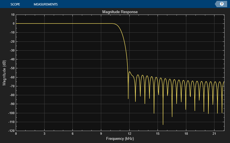
Change the background color and the axes color of the plot to "white". Set the font color to "black" and the line color to "blue".
dfv.BackgroundColor = "white";
dfv.AxesColor = "white";
dfv.FontColor = "black";
dfv.LineColor = "blue";
show(dfv)
release(dfv)
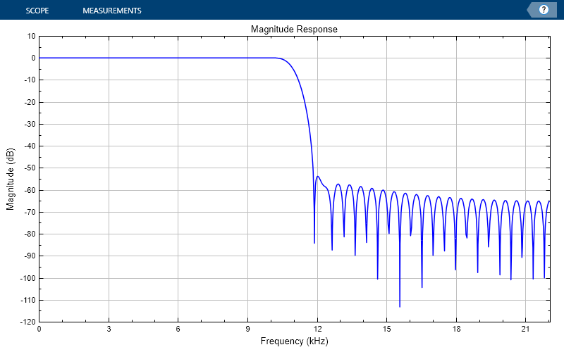
Print the display of the magnitude response to a new MATLAB figure. The function returns a handle to the figure.
scopeFig = printToFigure(dfv);

The handle to the figure scopeFig lets you modify the appearance and the behavior of the figure window.
Specify a figure name and change the size of the figure to 400-by-250 pixels.
scopeFig.Name="Magnitude Response of FIR Filter";
scopeFig.NumberTitle="off";
scopeFig.Position=[1 1 400 250];
When printing to figure, you can make the figure invisible by setting the Visible argument to false.
scopeFig = printToFigure(dfv,Visible=false);
Input Arguments
Output Arguments
Version History
Introduced in R2023b