spectrumAnalyzer
Description
The spectrumAnalyzer object displays frequency-domain signals and
the frequency spectrum of time-domain signals. The scope shows the spectrum view and the
spectrogram view. The object performs spectral estimation using the filter bank method and
Welch's method of averaged modified periodograms. You can customize the spectrum analyzer
display to show the data and the measurement information that you need. For more details, see
Algorithms. The spectrum analyzer can display
the power spectrum of the signal in three units, Watts,
dBm, and dBW. For more information on
how to convert the power within these three units, see Convert the Power Between Units.
To display the spectra of signals in the spectrum analyzer:
Create the
spectrumAnalyzerobject and set its properties.Call the object with arguments as if it were a function.

Creation
Description
scope = spectrumAnalyzer creates a
spectrumAnalyzer object that displays the frequency spectrum of real or
complex signals.
scope = spectrumAnalyzer(Name=Value) specifies nondefault
properties for scope using one or more name-value arguments. For example,
to display both spectrum and spectrogram, set ViewType to
"spectrum-and-spectrogram".
Properties
Frequently Used
The domain of the input signal you want to visualize, specified as
"time" or "frequency". If you want to
visualize time-domain signals, the spectrum analyzer transforms the signal to the
frequency spectrum based on the algorithm you specify in the Method property.
Scope Window Use
In the Estimation tab on the spectrum analyzer toolstrip,
set Input Domain to Time or
Frequency.
Data Types: char | string
The type of spectrum to display, specified as one of the following:
"power"— Power spectrum."power-density"— Power spectral density. The power spectral density is the squared magnitude of the spectrum normalized to a bandwidth of 1 hertz."rms"— Root mean square. The root-mean-square shows the square root of the mean square. Use this option to view the frequency of voltage or current signals.
Tunable: Yes
Dependency
To enable this property, set InputDomain to "time".
Scope Window Use
In the Scope tab on the spectrum analyzer toolstrip, click
the drop down arrow of Spectrum to select
Power, Power Density, or
RMS.
To enable these options, set the Input Domain on the
Estimation tab to Time.
Data Types: char | string
View to display, specified as one of the following:
"spectrum"— Display the frequency spectrum of signals."spectrogram"— Display the spectrogram of signals. Spectrogram shows the frequency content over time. Each line of the spectrogram is one periodogram. Time scrolls from the top to the bottom of the display. The most recent spectrogram update is at the top of the display."spectrum-and-spectrogram"— Display both spectrum and spectrogram.
To learn more about how the spectrum analyzer computes spectrum and spectrogram, see the Algorithms section.
Tunable: Yes
Scope Window Use
In the Scope tab on the spectrum analyzer toolstrip, select Spectrum, Spectrogram, or both.
Data Types: char | string
The sample rate of the input in Hz, specified as a positive scalar.
Tunable: Yes
Scope Window Use
Click the Scope tab on the spectrum analyzer toolstrip. In the Bandwidth section, specify Sample Rate (Hz) to a finite scalar.
The spectrum analyzer shows the sample rate in the status bar at the bottom of the display.
Data Types: double
Spectrum estimation method, specified as one of the following:
"filter-bank"–– Use an analysis filter bank to estimate the power spectrum. Compared to Welch's method, this method has a lower noise floor, better frequency resolution, and lower spectral leakage and requires fewer samples per update."welch"–– Use Welch's method of averaged modified periodograms.
For more details on these methods, see Algorithms.
Tunable: Yes
Dependency
To enable this property, set InputDomain to "time".
Scope Window Use
In the Estimation tab of the spectrum analyzer toolstrip,
set Estimation Method to Filter bank
or Welch.
To enable this parameter, set Input Domain to
Time in the Estimation tab.
Data Types: char | string
Option to plot a two-sided spectrum, specified as one of the following:
true— Compute and plot two-sided spectral estimates. When the input signal is complex valued, you must set this property totrue.false— Compute and plot one-sided spectral estimates. If you set this property tofalse, then the input signal must be real valued.When you set this property to
false, the Spectrum Analyzer uses power-folding. The y-axis values are twice the amplitude that they would be if you were to set this property totrue, except at0and the Nyquist frequency. A one-sided power spectral density (PSD) contains the total power of the signal in the frequency interval from DC to half the Nyquist rate. For more information, seepwelch.
Tunable: Yes
Scope Window Use
Click the Spectrum tab or the Spectrogram tab (if enabled) of the Spectrum Analyzer toolstrip. In the Trace Options section, select Two-Sided Spectrum to compute and plot two-sided spectral estimates.
Data Types: logical
Scale to display frequency, specified as one of the following:
"linear"— Use a linear scale to display frequencies on the x-axis."log"— Use a logarithmic scale to display frequencies on the x-axis.
Tunable: Yes
Dependency
To set this property to "log", set the
PlotAsTwoSidedSpectrum property to
false.
Scope Window Use
Click the Spectrum tab or the
Spectrogram tab (if enabled) of the spectrum analyzer
toolstrip. In the Scale section, set the Frequency
Scale to Linear or
Log.
To set the Frequency Scale to
Log, clear the Two-Sided Spectrum
check box in the Trace Options section in the
Spectrum or the Spectrogram tab (if
enabled). If you select the Two-Sided Spectrum check box, then
you must set the Frequency Scale to
Linear.
Data Types: char | string
Type of plot to use for displaying normal traces, specified as
"line", "stem", or a cell array of these
character vectors, or an array of strings. Normal traces are traces that display
free-running spectral estimates.
You can individually control the type of
plot for each line by specifying the PlotType property as a cell
array of character vectors or an array of strings. (since R2025a)
Tunable: Yes
Dependencies
To enable this property, set:
ViewTypeto"spectrum"or"spectrum-and-spectrogram".PlotNormalTracetotrue.
Scope Window Use
Click the Scope tab on the spectrum analyzer toolstrip,
navigate to the Configuration section and click
Settings. In the Spectrum Analyzer Settings window that
opens, set Plot Type to Line or
Stem.
To enable the Plot Type, you must:
Select Spectrum in the Views section of the Scope tab.
Enable the Normal Trace check box in the Trace Options section of the Spectrum tab.
Data Types: char | string
Axes scaling mode, specified as one of the following:
"auto"— The scope scales the axes to fit the data, both during and after simulation."manual"— The scope does not scale the axes automatically."onceatstop"— The scope scales the axes when the simulation stops and you call thereleasefunction."updates"— The scope scales the axes after a specific number of visual updates. It determines the number of updates using theAxesScalingNumUpdatesproperty.
Tunable: Yes
Data Types: char | string
Number of updates before scaling, specified as a positive integer.
Tunable: Yes
Dependency
To enable this property, set AxesScaling to "updates".
Data Types: double
Advanced
Frequency resolution method of the spectrum analyzer, specified as one of these options:
"rbw"–– TheRBWSourceandRBWproperties control the frequency resolution (in Hz) of the analyzer."num-frequency-bands"–– Applies only when you setMethodto"filter-bank". TheFFTLengthSourceandFFTLengthproperties control the frequency resolution."window-length"–– Applies only when you setMethodto"welch". TheWindowLengthproperty controls the frequency resolution.
Tunable: Yes
Dependency
To enable this property, set InputDomain to
"time".
Scope Window Use
Click the Estimation tab on the Spectrum Analyzer toolstrip. In the Frequency Resolution section, set Resolution Method to one of the available options.
Data Types: char | string
The source of the resolution bandwidth (RBW), specified as
"auto" or "property".
"auto"— The spectrum analyzer adjusts the spectral estimation resolution to ensure that there are 1024 RBW intervals over the defined frequency span."property"— Specify the resolution bandwidth directly using theRBWproperty.
Tunable: Yes
Dependency
To enable this property, set FrequencyResolutionMethod to
"rbw".
Scope Window Use
Click the Estimation tab on the spectrum analyzer
toolstrip. In the Frequency Resolution section, set
RBW (Hz) to either Auto or a
positive scalar.
Data Types: char | string
Resolution bandwidth (RBW) in Hz, specified as a positive scalar. Specify the value to ensure that there are at least two RBW intervals over the specified frequency span. The ratio of the overall span to RBW satisfies this condition:
Specify the overall span based on how you set the FrequencySpan property.
RBW controls the spectral resolution of the displayed signal. The RBW value determines the spacing between frequencies that can be resolved. A smaller value gives a higher spectral resolution and lowers the noise floor. That is, the spectrum analyzer can resolve frequencies that are closer to each other. However, this comes at the cost of a longer sweep time.
Dependency
To enable this property, set RBWSource to "property".
Scope Window Use
Click the Estimation tab on the spectrum analyzer toolstrip. In the Frequency Resolution section, set RBW (Hz) to a positive scalar.
The spectrum analyzer shows the value of RBW in the status bar at the bottom of the display.
Tunable: Yes
Data Types: double
Since R2024a
Window length in samples that the object uses to compute the spectral estimates, specified as an integer greater than 2. This property controls the frequency resolution.
Tunable: Yes
Dependencies
To enable this property, set:
Methodto"welch".FrequencyResolutionMethodto"window-length".
Scope Window Use
Click the Estimation tab on the spectrum analyzer toolstrip. In the Frequency Resolution section, set the Window Length to a positive integer greater than 2.
To enable Window Length, set:
Estimation Method to
Welch.Resolution Method to
Window length.
Since R2024b
Set this property to true to maintain the number of samples per
update Nsamples at 1024 regardless of the
window you select in the Window property. The RBW value adjusts
according to the window you select.
where:
Op is the overlap percentage you specify in the
OverlapPercentproperty.Fs is the sample rate you specify using the
SampleRateSourceandSampleRateproperties.RBW is the resolution bandwidth you specify in the
RBWSourceandRBWproperties.NENBW is the normalized effective noise bandwidth. For more information, see the Spectrum Analyzer block reference page.
When you set this parameter to false, the object maintains the
same RBW value and adjusts the number of samples required per update
Nsamples depending on the window you
select.
Dependencies
To enable this property, set:
Methodto"welch".FrequencyResolutionMethodto"rbw".RBWSourceto"auto".
Tunable: Yes
Data Types: logical
Source of the FFT length, specified as one of these:
"auto"–– The value of FFT length depends on the setting of the frequency resolution method. When you set:FrequencyResolutionMethodto"rbw", the FFT length equals the number of samples per update, Nsamples. For more details on Nsamples, see the Algorithms section.FrequencyResolutionMethodto"window-length", the FFT length equals the value you specify in theWindowLengthproperty or 1024, whichever is larger.FrequencyResolutionMethodto"num-frequency-bands", the FFT length equals the input frame size (number of rows).
"property"–– The number of FFT points equals the value you specify in theFFTLengthproperty.
Tunable: Yes
Dependency
To enable this property, set:
Methodto"welch".Methodto"filter-bank"andFrequencyResolutionMethodto"num-frequency-bands".
Scope Window Use
Click the Estimation tab on the spectrum analyzer toolstrip.
In the Frequency Resolution section, set the FFT
Length to Auto or a positive
integer.
Data Types: char | string
Since R2024a
Length of the FFT that the spectrum analyzer uses to compute spectral estimates, specified as a positive integer.
Tunable: Yes
Dependencies
To enable this property, set FFTLengthSource to
"property".
Scope Window Use
Click the Estimation tab on the spectrum analyzer
toolstrip. In the Frequency Resolution section, set the
FFT Length to Auto or a positive
integer.
Sharpness of the prototype lowpass filter, specified as a real nonnegative scalar in the range [0,1].
Increasing the filter sharpness decreases the spectral leakage and gives a more accurate power reading.
Tunable: Yes
Dependencies
To enable this property, set Method to "filter-bank".
Scope Window Use
Click the Estimation tab on the spectrum analyzer toolstrip. In the Frequency Resolution section, set Filter Sharpness.
To enable this parameter, set Input Domain to
Time in the Estimation tab.
Data Types: double
Source of the frequency vector, specified as one of the following:
"auto"— The spectrum analyzer computes the frequency vector based on the frame size of the input signal and the specified sample rate."property"— Enter a custom vector in theFrequencyVectorproperty.
Tunable: Yes
Dependency
To enable this property, set InputDomain to "frequency".
Scope Window Use
Click the Estimation tab on the spectrum analyzer
toolstrip. In the Domain section, set Frequency
(Hz) to either Auto or a monotonically
increasing vector of length equal to the input signal frame size.
To enable the Frequency (Hz), set Input
Domain to Frequency.
Data Types: char | string
Custom frequency vector, specified as a monotonically increasing vector. This vector determines the x-axis of the display. The vector must be monotonically increasing and must have the same length as the input signal frame size.
Tunable: Yes
Dependency
To enable this property, set:
InputDomainto"frequency".FrequencyVectorSourceto"property".
Scope Window Use
Click the Estimation tab on the spectrum analyzer
toolstrip. In the Domain section, set Frequency
(Hz) to either Auto or a monotonically
increasing vector of length equal to the input signal frame size.
To enable the Frequency (Hz), set Input
Domain to Frequency.
Data Types: double
Frequency span mode, specified as one of the following:
"full"–– The spectrum analyzer computes and plots the spectrum over the entire Nyquist Frequency Interval."span-and-center-frequency"–– The spectrum analyzer computes and plots the spectrum over the interval specified by theSpanandCenterFrequencyproperties."start-and-stop-frequencies"–– The spectrum analyzer computes and plots the spectrum over the interval specified by theStartFrequencyandStopFrequencyproperties.
Tunable: Yes
Dependency
To enable this property, set InputDomain to "time".
Scope Window Use
Click the Estimation tab on the spectrum analyzer
toolstrip. In the Frequency Options section, set
Frequency Span to Full,
Span and Center Frequency, or Start and
Stop Frequencies.
To enable the Frequency Span, set Input
Domain to Time.
Data Types: char | string
Frequency span over which the spectrum analyzer computes and plots the spectrum,
specified as a positive scalar in Hz. The overall span, defined by this property and
the CenterFrequency property, must fall within the Nyquist Frequency Interval.
Tunable: Yes
Dependency
To enable this property, set:
InputDomainto"time"FrequencySpanto"span-and-center-frequency"
Scope Window Use
Click the Estimation tab on the spectrum analyzer
toolstrip. In the Frequency Options section, set
Frequency Span to Span and Center
Frequency and Span (Hz) to a positive
scalar.
To enable the Frequency Span, set Input
Domain to Time.
Data Types: double
Center of frequency span over which the spectrum analyzer computes and plots the
spectrum, specified as a real scalar in Hz. The overall frequency span, defined by
Span and this property, must fall within the Nyquist Frequency Interval.
Tunable: Yes
Dependency
To enable this property, set:
InputDomainto"time"FrequencySpanto"span-and-center-frequency"
Scope Window Use
Click the Estimation tab on the spectrum analyzer
toolstrip. In the Frequency Options section, set
Frequency Span to Span and Center
Frequency and Center Frequency (Hz) to a real
scalar.
To enable the Frequency Span, set Input
Domain to Time.
Data Types: double
Starting frequency in the frequency interval over which the spectrum analyzer
computes and plots the spectrum, specified as a real scalar in Hz. The overall span,
which is defined by this property and StopFrequency, must fall within the Nyquist Frequency Interval.
Tunable: Yes
Dependency
To enable this property, set:
InputDomainto"time"FrequencySpanto"start-and-stop-frequencies"
Scope Window Use
Click the Estimation tab on the spectrum analyzer
toolstrip. In the Frequency Options section, set
Frequency Span to Start and Stop
Frequencies and Start Frequency (Hz) to a real
scalar.
To enable the Frequency Span, set Input
Domain to Time.
Data Types: double
Ending frequency in the frequency interval over which the spectrum analyzer
computes and plots the spectrum, specified as a real scalar in Hz. The overall span,
which is defined by this property and the StartFrequency property, must fall within the Nyquist Frequency Interval.
Tunable: Yes
Dependency
To enable this property, set:
InputDomainto"time"FrequencySpanto"start-and-stop-frequencies"
Scope Window Use
Click the Estimation tab on the spectrum analyzer
toolstrip. In the Frequency Options section, set
Frequency Span to Start and Stop
Frequencies and Stop Frequency (Hz) to a real
scalar.
To enable the Frequency Span, set Input
Domain to Time.
Data Types: double
Percentage of overlap between the previous and current buffered data segments, specified as a scalar in the range [0 100). The overlap creates a window segment that the object uses to compute a spectral estimate.
Tunable: Yes
Dependency
To enable this property, set:
InputDomainto"time"Methodto"welch"
Scope Window Use
Click the Estimation tab on the spectrum analyzer toolstrip. In the Window Options section, set the Overlap (%).
To enable the Overlap (%), set Input
Domain to Time and Estimation
Method to Welch in the
Estimation tab on the spectrum analyzer toolstrip.
Data Types: double
Window function, specified as one of the following preset windows. For more information on a window option, click the link to the corresponding function.
| Window Option | Corresponding Signal Processing Toolbox™ Function |
|---|---|
"hann" | hann |
"blackman-harris" | blackmanharris |
"chebyshev" | chebwin |
"flat-top" | flattopwin |
"hamming" | hamming |
"kaiser" | kaiser |
"rectangular" | rectwin |
To use your own spectral estimation window, set this property to
"custom" and specify a custom window function in the CustomWindow property.
Tunable: Yes
Dependency
To enable this property, set:
InputDomainto"time"Methodto"welch"
Scope Window Use
Click the Estimation tab on the spectrum analyzer toolstrip. In the Window Options section, set the Window.
To enable the Window, set Input Domain
to Time and Estimation Method to
Welch in the Estimation tab on the
spectrum analyzer toolstrip.
Data Types: char | string
Name of custom window function, specified as a character array or string scalar. The custom window function name must be on the MATLAB® path. Use this property to customize a window function using additional properties available with the Signal Processing Toolbox.
Tunable: Yes
Example:
Define and use a custom window function.
function w = my_hann(L) w = hann(L,"periodic") end scope.Window = "custom"; scope.CustomWindow = "my_hann"
Dependency
To use this property, set Window to "custom".
Scope Window Use
Click the Estimation tab on the spectrum analyzer toolstrip. In the Window Options section, for the Window, enter a custom window function name.
Data Types: char | string
Sidelobe attenuation of the window in decibels (dB), specified as a positive
scalar greater than or equal to 45.
Tunable: Yes
Dependency
To enable this property, set Window to "chebyshev" or
"kaiser".
Scope Window Use
Click the Estimation tab on the spectrum analyzer toolstrip. In the Window Options section, set the Attenuation (dB).
To enable the Attenuation (dB), set:
Input Domain to
TimeEstimation Method to
WelchWindow to either
ChebyshevorKaiserin the Estimation tab on the spectrum analyzer toolstrip.
Data Types: double
Averaging method, specified as one of these:
"vbw"— Video bandwidth method. The object uses a lowpass filter to smooth the trace and decrease noise. Use theVBWSourceandVBWproperties to specify the VBW value."exponential"— Weighted average of samples. The object computes the average over samples weighted by an exponentially decaying forgetting factor. Use theForgettingFactorproperty to specify the weighted forgetting factor."running"–– Running average of the last Q samples. Use theSpectralAveragesproperty to specify Q. (since R2025a)
For more information on averaging methods, see Averaging Method.
Tunable: Yes
Dependency
To enable this property, set InputDomain to "time".
Scope Window Use
Click the Estimation tab on the spectrum analyzer
toolstrip. In the Averaging section, set Averaging
Method to VBW,
Exponential, or
Running.
To enable the Averaging Method, set Input
Domain to Time.
Data Types: char | string
Forgetting factor of the exponential weighted averaging method, specified as a scalar in the range [0,1].
Tunable: Yes
Dependency
To enable this property, set:
InputDomainto"time".AveragingMethodto"exponential"
Scope Window Use
Click the Estimation tab on the spectrum analyzer toolstrip. In the Averaging section, set Forgetting Factor.
To enable the Forgetting Factor, set Input
Domain to Time and Averaging
Method to Exponential.
Data Types: double
Source of the video bandwidth (VBW), specified as either "auto"
or "property".
"auto"— The spectrum analyzer adjusts the VBW such that the equivalent forgetting factor is 0.9."property"— The spectrum analyzer adjusts the VBW using the value specified in theVBWproperty.
For more details on the video bandwidth method, see Averaging Method.
Tunable: Yes
Dependency
To enable this property, set InputDomain to "time" and AveragingMethod to vbw.
Scope Window Use
Click the Estimation tab on the spectrum analyzer
toolstrip. In the Averaging section, set VBW
(Hz) to either Auto or a positive real
scalar less than or equal to Sample Rate (Hz)/2.
To enable the VBW (Hz), set Input
Domain to Time and Averaging
Method to VBW.
Data Types: char | string
Video bandwidth, specified as a positive scalar less than or equal to SampleRate/2. For more details on the video bandwidth method, see Averaging Method.
The spectrum analyzer shows the value of VBW in the status bar at the bottom of the display.
Tunable: Yes
Dependency
To enable this property, set VBWSource to "property".
Scope Window Use
Click the Estimation tab on the spectrum analyzer
toolstrip. In the Averaging section, set VBW
(Hz) to either Auto or enter a positive real
scalar that is less than or equal to Sample Rate (Hz)/2.
To enable the VBW (Hz), set Input
Domain to Time and Averaging
Method to VBW.
Data Types: double
Since R2025a
Number of spectral averages Q, specified as a positive integer.
The spectrum analyzer computes the current power spectrum estimate by computing a running average of the last Q power spectrum estimates.
Dependency
To enable this property, set:
InputDomainto"time".AveragingMethodto"running".
Scope Window Use
Click the Estimation tab on the spectrum analyzer
toolstrip. In the Averaging section, set Averaging
Method to Running and Spectral
Averages to a positive integer.
To enable the Averaging Method, set Input
Domain to Time.
Data Types: double
Units of the frequency-domain input, specified as "dBm",
"dBuV" (since R2023b),
"dBV", "dBW", "Vrms",
"Watts", or "none". The spectrum analyzer
scales frequency data according to the display unit.
Tunable: Yes
Dependency
To enable this property, set InputDomain to "frequency".
Scope Window Use
Click the Estimation tab on the spectrum analyzer toolstrip. In the Domain section, set Input Unit.
To enable the Input Unit, set Input
Domain to Frequency.
Data Types: char | string
Units of the spectrum, specified as one of the following:
"dBm""dBFS""dBuV"(since R2023b)"dBV""dBW""Vrms""Watts""dBm/Hz""dBW/Hz""dBFS/Hz""Watts/Hz""auto"
Tunable: Yes
Dependency
The available spectrum units depend on the value you specify in the SpectrumType property.
InputDomain | SpectrumType | Allowed SpectrumUnits |
|---|---|---|
"time" | "power" | "dBm", "dBW",
"dBFS", "Watts" |
"power-density" | "dBm/Hz",
"dBW/Hz","dBFS/Hz",
"Watts/Hz" | |
"rms" | "dBuV" (since R2023b),
"dBV", "Vrms" | |
"frequency" | ― | "auto", "dBm", "dBuV" (since R2023b),
"dBV", "dBW",
"Vrms", "Watts" |
If you set the InputDomain property to
"frequency" and the SpectrumUnits property
to "auto", the spectrum analyzer assumes the spectrum units to be
equal to input units specified in the InputUnits property. If you set InputDomain to
"time" and SpectrumUnits to any option
other than "auto", the spectrum analyzer converts the units
specified in InputUnits to the units specified in
SpectrumUnits.
Scope Window Use
Click the Spectrum tab on the spectrum analyzer toolstrip. In the Scale section, set Spectrum Unit.
Data Types: char | string
Source of the dBFS scaling factor, specified as either "auto"
or "property".
"auto"–– The spectrum analyzer adjusts the scaling factor based on the input data."property"–– Specify the full-scale scaling factor using theFullScaleproperty.
Tunable: Yes
Dependency
To enable this property, set:
InputDomainto"time"SpectrumTypeto"power"or"power-density"SpectrumUnitsto"dBFS"or"dBFS/Hz"
Scope Window Use
Click the Spectrum tab on the spectrum analyzer toolstrip.
In the Scale section, set the Full Scale
to either Auto or a positive scalar.
To enable the Full Scale:
In the Scope tab, set the spectrum type to
PowerorPower Density.In the Estimation tab, set Input Domain to
Time.In the Spectrum tab, set Spectrum Unit to
dBFSordBFS/Hz(when spectrum type is set toPower Density).
Data Types: char | string
dBFS full scale, specified a positive scalar.
Tunable: Yes
Dependency
To enable this property, set:
InputDomainto"time"SpectrumTypeto"power"or"power-density"SpectrumUnitsto"dBFS"or"dBFS/Hz"FullScaleSourceto"property"
Scope Window Use
Click the Spectrum tab on the spectrum analyzer toolstrip.
In the Scale section, set the Full Scale
to either Auto or enter a positive scalar.
To enable the Full Scale:
In the Scope tab, set the spectrum type to
PowerorPower Density.In the Estimation tab, set Input Domain to
Time.In the Spectrum tab, set Spectrum Unit to
dBFSordBFS/Hz(when spectrum type is set toPower Density).
Data Types: double
Load that the scope uses as a reference to compute power levels, specified as a positive scalar in Ohms.
Tunable: Yes
Dependency
To enable this property, set:
SpectrumTypeto"power"or"power-density".SpectrumUnitsto any option other than"dBFS"or"dBFS/Hz".
Scope Window Use
Click the Spectrum tab on the spectrum analyzer toolstrip. In the Scale section, set Reference Load (Ω).
Data Types: double
Offset to apply to the frequency axis (x-axis) in units of Hz, specified as one of the following:
Scalar — Apply the same frequency offset to all channels.
Vector — Apply a specific frequency offset for each channel. The vector length must be equal to the number of input channels.
The overall span must fall within the Nyquist Frequency Interval. You can control the overall span in different ways based on how you set the
FrequencySpanproperty.
Tunable: Yes
Scope Window Use
Click the Scope tab on the spectrum analyzer toolstrip. In the Bandwidth section, set Offset (Hz).
Data Types: double
Spectrogram
Channel for which the spectrogram is plotted, specified as a positive integer in the range [1 N], where N is the number of input channels.
Tunable: Yes
Dependency
To enable this property, set ViewType to "spectrogram" or
"spectrum-and-spectrogram".
Scope Window Use
Click the Spectrogram tab on the spectrum analyzer toolstrip. In the Channel section, select a Channel.
Data Types: double
Since R2026a
Orientation of time in spectrogram, specified as one of these:
"vertical"— Time is on the y-axis and frequency is on the x-axis. As the simulation progresses, the spectrogram scrolls in the vertical direction from top to bottom."horizontal"— Time is on the x-axis and frequency is on the y-axis. As the simulation progresses, the spectrogram scrolls in the horizontal direction from right to left.
Tunable: Yes
Dependency
To enable this property, set ViewType to "spectrogram" or
"spectrum-and-spectrogram".
Scope Window Use
Click the Spectrogram tab on the spectrum analyzer
toolstrip. In the Time Options section, set the Time
Orientation to Vertical or
Horizontal.
Data Types: char | string
Source of the time resolution of each spectrogram line, specified as either
"auto" or "property".
When you set RBWSource and TimeResolutionSource to
"auto", then RBW is set such that there are 1024 RBW intervals in
one frequency span. The time resolution is set to 1/RBW.
When RBWSource is set to "auto" and
TimeResolutionSource is set to "property",
then time resolution becomes the main control and RBW is set to 1/TimeResolution Hz.
When RBWSource is set to "property" and
TimeResolutionSource is set to "auto", then
RBW becomes the main control and the time resolution is set 1/RBW s.
When both RBWSource and
TimeResolutionSource are set to "property",
then the specified time resolution value must be equal to or larger than the minimum
attainable time resolution which is defined by 1/RBW. Several spectral estimates are
combined into one spectrogram line to obtain the desired time resolution.
Tunable: Yes
Dependency
To enable this property, set:
InputDomainto"time".ViewTypeto"spectrogram"or"spectrum-and-spectrogram".
Scope Window Use
Click the Spectrogram tab on the spectrum analyzer
toolstrip. In the Time Options section, set the Time
Resolution (s) to Auto or enter a positive
scalar.
To enable the Time Resolution (s), select
Spectrogram in the Scope tab and set
Input Domain to Time in the
Estimation tab.
Data Types: char | string
Time resolution of each spectrogram line in seconds, specified as a positive scalar.
Tunable: Yes
Dependency
To enable this property, set:
InputDomainto"time".ViewTypeto"spectrogram"or"spectrum-and-spectrogram".TimeResolutionSourceto"property".
Scope Window Use
Click the Spectrogram tab on the spectrum analyzer
toolstrip. In the Time Options section, set the Time
Resolution (s) to Auto or enter a positive
scalar.
To enable the Time Resolution (s), select
Spectrogram in the Scope tab and set
Input Domain to Time in the
Estimation tab.
Data Types: double
Source for the time span of the spectrogram, specified as either one of these:
"auto"–– The spectrogram displays 100 spectrogram lines at any given time."property"–– The spectrogram uses the time duration you specify in seconds in theTimeSpanproperty.The time span that you specify must be at least two times larger than the duration of the number of samples required for a spectral update.
Tunable: Yes
Dependency
To enable this property, set ViewType to "spectrogram" or
"spectrum-and-spectrogram".
Scope Window Use
Click the Spectrogram tab on the spectrum analyzer
toolstrip. In the Time Options section, set the Time
Span (s) to Auto or enter a positive scalar.
Data Types: char | string
Time span of the spectrogram display in seconds, specified as a positive scalar. You must set the time span to be at least twice as large as the duration of the number of samples required for a spectral update.
Tunable: Yes
Dependency
To enable this property, set:
ViewTypeto"spectrogram"or"spectrum-and-spectrogram".TimeSpanSourceto"property".
Scope Window Use
Click the Spectrogram tab on the spectrum analyzer
toolstrip. In the Time Options section, set the Time
Span (s) to Auto or enter a positive scalar.
Data Types: double
Measurements
The channel for which you need to obtain measurements, specified as a positive integer in the range [1 N], where N is the number of input channels.
Tunable: Yes
Scope Window Use
Click the Measurements tab on the spectrum analyzer toolstrip. In the Channel section, select a Channel.
Data Types: double
Channel measurements, specified as a ChannelMeasurementsConfiguration object. Enable channel measurements to
compute and display the occupied bandwidth or adjacent channel power ratio. All
ChannelMeasurementsConfiguration properties are tunable.
Tunable: Yes
Dependency
To enable this property, set ViewType to either "spectrum" or
"spectrum-and-spectrogram".
Scope Window Use
Click the Channel Measurements tab on the spectrum analyzer toolstrip and modify the measurement settings.
The Channel Measurements tab appears when you select Spectrum in the Scope tab.
Cursor measurements, specified as a CursorMeasurementsConfiguration object. Enable cursor measurements to
display waveform cursors. All CursorMeasurementsConfiguration
properties are tunable.
Tunable: Yes
Scope Window Use
Click the Measurements tab on the spectrum analyzer toolstrip and modify the cursor measurements in the Cursors section.
Distortion measurements, specified as a DistortionMeasurementsConfiguration object. Enable distortion measurements
to compute and display the harmonic distortion and intermodulation distortion. All
DistortionMeasurementsConfiguration properties are tunable. For
more details, see Distortion Measurements and Harmonic Measurements.
Tunable: Yes
Dependency
To enable this property, set ViewType to either "spectrum" or
"spectrum-and-spectrogram".
Scope Window Use
Click the Measurements tab on the spectrum analyzer toolstrip and modify the distortion measurements in the Distortion section.
Peak finder measurements, specified as a PeakFinderConfiguration object. Enable peak finder to compute and display
the largest calculated peak values. All PeakFinderConfiguration
properties are tunable.
Tunable: Yes
Dependency
To enable this property, set ViewType to either "spectrum" or
"spectrum-and-spectrogram".
Scope Window Use
Click the Measurements tab on the spectrum analyzer toolstrip and modify the peak finder measurements in the Peaks section.
Since R2025a
Phase noise measurements, specified as a PhaseNoiseConfiguration object. Enable the PhaseNoise
property to measure the phase noise of the signal and plot it against the specified
target phase noise profile. All PhaseNoiseConfiguration properties
are tunable.
Note
To measure the phase noise, you must have a valid Mixed-Signal Blockset™ license.
Tunable: Yes
Scope Window Use
Click the Measurements tab on the spectrum analyzer toolstrip and modify the phase noise measurement settings in the Phase Noise section.
Spectral mask configuration, specified as a SpectralMaskConfiguration object. Use the spectral mask configuration to
draw upper and lower or upper or lower mask lines in the power and power-density
plots. All SpectralMaskConfiguration properties are tunable.
Tunable: Yes
Dependency
To enable this property, set:
ViewTypeto either"spectrum"or"spectrum-and-spectrogram".SpectrumTypeto either"power"or"power-density".
Scope Window Use
Click the Spectral Mask tab on the spectrum analyzer toolstrip and modify the settings.
The Spectral Mask tab appears when you:
Select Spectrum in the Scope tab.
In the drop-down list under Spectrum, choose either
PowerorPower Density.
Visualization
Caption to display in the scope window, specified as a character vector or string scalar.
Tunable: Yes
Data Types: char | string
Spectrum analyzer window position in pixels, specified as a four-element double
vector of the form [left bottom width height]. You can place the
scope window in a specific position on your screen by modifying the values of this
property.
By default, the window appears at the center of your screen with a width of
800 pixels and height of 500 pixels. The exact
center coordinates depend on your screen resolution.
Tunable: Yes
Maximize axes control, specified as one of the following:
"auto"–– The spectrum analyzer maximizes axes only if the display does not contain any labels or title annotations."on"–– The spectrum analyzer maximizes axes in all displays."off"–– The spectrum analyzer does not maximize axes in any display.
Tunable: Yes
Data Types: char | string
To remove normal traces from the display, set this property to
false. These traces display the free-running spectral estimates.
The spectrum analyzer continues its spectral computations even when you set this
property to false.
Tunable: Yes
Dependency
To enable this property, set ViewType to "spectrum" or
"spectrum-and-spectrogram".
Scope Window Use
Click the Spectrum tab on the spectrum analyzer toolstrip and select the Normal Trace check box in the Trace Options section.
To enable the Normal Trace check box, select Spectrum in the Scope tab.
Data Types: logical
Option to plot max-hold trace, specified as true or
false. To compute and plot the maximum-hold spectrum of each
input channel, set this property to true. The spectrum analyzer
computes the maximum-hold spectrum at each frequency bin by keeping the maximum value
of all the power spectrum estimates. When you change the value of this property, the
spectrum analyzer resets its maximum-hold computations.
Tunable: Yes
Dependency
To enable this property, set ViewType to "spectrum" or
"spectrum-and-spectrogram".
Scope Window Use
Click the Spectrum tab on the spectrum analyzer toolstrip and select the Max-Hold Trace check box in the Trace Options section.
To enable the Max-Hold Trace check box, select Spectrum in the Scope tab.
Data Types: logical
Option to plot min-hold trace, specified as true or
false. To compute and plot the minimum-hold spectrum of each
input channel, set this property to true. The spectrum analyzer
computes the minimum-hold spectrum at each frequency bin by keeping the minimum value
of all the power spectrum estimates. When you change the value of this property, the
spectrum analyzer resets its minimum-hold computations.
Tunable: Yes
Dependency
To enable this property, set ViewType to "spectrum" or
"spectrum-and-spectrogram".
Scope Window Use
Click the Spectrum tab on the spectrum analyzer toolstrip and select the Min-Hold Trace check box in the Trace Options section.
To enable the Min-Hold Trace check box, select Spectrum in the Scope tab.
Data Types: logical
Display title, specified as a character vector or a string scalar.
Tunable: Yes
Scope Window Use
Click the Scope tab on the spectrum analyzer toolstrip. In the Configuration section, click Settings, and enter Title.
Data Types: char | string
y-axis label, specified as a character vector or a string scalar. The spectrum analyzer displays the label to the left of the y-axis.
Regardless of this property, spectrum analyzer always displays power units as one
of the SpectrumUnits values.
Tunable: Yes
Dependency
To enable this property, set ViewType to "spectrum" or
"spectrum-and-spectrogram".
Scope Window Use
Click the Scope tab on the spectrum analyzer toolstrip. In the Configuration section, click Settings, and enter Y-Label.
To enable the Y-Label, select Spectrum in the Scope tab.
Data Types: char | string
y-axis limits, specified as a two-element numeric vector of the
form [ymin ymax]. The units of the y-axis limits
depend on the SpectrumUnits property.
Example: scope.YLimits = [-10,20]
Tunable: Yes
Dependencies
To enable this property, set the ViewType property to "spectrum" or
"spectrum-and-spectrogram".
Scope Window Use
Click the Scope tab on the spectrum analyzer toolstrip. In the Configuration section, click Settings, and enter Y-Limits.
To enable the Y-Limits, select Spectrum in the Scope tab.
Color limits of the spectrogram, specified as a two-element numeric vector of the
form [colorMin colorMax]. The units of the color limits directly
depend upon the SpectrumUnits property.
Example: scope.ColorLimits = [-10,20]
Tunable: Yes
Dependencies
To enable this property, set the ViewType property to "spectrogram" or
"spectrum-and-spectrogram".
Scope Window Use
Click the Scope tab on the spectrum analyzer toolstrip. In the Configuration section, click Settings, and enter Color Limits.
To enable the Color Limits, select Spectrogram in the Scope tab.
Color look-up table, specified as a valid colormap name or a three-column matrix with values in the range [0,1] defining RGB triplets.
Tunable: Yes
Dependencies
To enable this property, set the ViewType property to "spectrogram" or
"spectrum-and-spectrogram".
Scope Window Use
Click the Scope tab on the spectrum analyzer toolstrip. In the Configuration section, click Settings, and enter Color Map.
To enable the Color Map, select Spectrogram in the Scope tab.
Data Types: double | char | string
Flag to show the grid, specified as true or
false. Set this property to true to show grid
lines in the plot.
Tunable: Yes
Scope Window Use
Click the Scope tab on the Spectrum Analyzer toolstrip. In the Configuration section, click Settings, and select Show Grid.
Data Types: logical
Show or hide the legend, specified as true or
false. To show a legend with the input names, set this property
to true.
Use the legend to control which signals are visible. In the scope legend, click a signal name to hide the signal in the scope. To show the signal, click the signal name again. To show only one signal, right-click the signal name. To show all signals, press Esc.
Tunable: Yes
Dependencies
To enable this property, set the ViewType property to "spectrum" or
"spectrum-and-spectrogram".
Scope Window Use
Click the Scope tab on the spectrum analyzer toolstrip. To see the legend, click Legend in the Configuration section.
To enable the Legend, select Spectrum in the Scope tab.
Data Types: logical
Show or hide color bar, specified as true or
false.
Tunable: Yes
Dependencies
To enable this property, set the ViewType property to "spectrogram" or
"spectrum-and-spectrogram".
Scope Window Use
Click the Scope tab on the spectrum analyzer toolstrip. To see the color bar, click Colorbar in the Configuration section.
To enable the Colorbar, select Spectrogram in the Scope tab.
Data Types: logical
Channel names in the input data, specified as a cell array of character vectors or an array of strings. The names you specify in this property appear in the following locations:
Legend
Spectrum Analyzer Settings > Color and styling section
Measurements and Channel Measurements tabs
If you do not specify channel names, the
spectrum analyzer names the channels as Channel 1, Channel
2, and so on.
Tunable: Yes
Dependency
To see the channel names, set ShowLegend to
true.
Scope Window Use
Click the Scope tab on the spectrum analyzer toolstrip. To see the legend, click Legend in the Configuration section.
Data Types: char
Layout of the axes, specified as one of "vertical" or
"horizontal". A vertical layout stacks the spectrum above the
spectrogram. A horizontal layout puts the two views side-by-side.
Tunable: Yes
Dependency
To enable this property, set ViewType to "spectrum-and-spectrogram".
Scope Window Use
Click the Scope tab on the spectrum analyzer toolstrip. Select Spectrum and Spectrogram. In the Configuration section, select and update Layout.
Data Types: char | string
Color and Styling
Since R2024b
Background color in scope, specified as an RGB triplet, a hexadecimal color code, a color name, or a short name. For more information on all the acceptable values, see Color.
Tunable: Yes
Scope Window Use
On the Scope tab, click Settings, and select a Background color.
Data Types: double | char
Since R2024b
Color of the axes in the scope, specified as an RGB triplet, a hexadecimal color code, a color name, or a short name. For more information on all the acceptable values, see Color.
Tunable: Yes
Scope Window Use
On the Scope tab, click Settings, and select an Axes color.
Data Types: double | char
Since R2024b
Colors of the labels in the scope, specified as an RGB triplet, a hexadecimal color code, a color name, or a short name. Use this property to set the color of the scope title, x-axis and y-axis labels, and the axes ticks. For more information on all the acceptable values, see Color.
Tunable: Yes
Scope Window Use
On the Scope tab, click Settings, and select a Labels color.
Data Types: double | char
Since R2024b
Scope font size, specified as a positive scalar. Use this property to set the font size for the ticks, labels, title, and measurements of the scope.
Tunable: Yes
Scope Window Use
On the Scope tab, click Settings, and set the Font Size to one of the available values.
Data Types: single | double | int8 | int16 | int32 | int64 | uint8 | uint16 | uint32 | uint64
Since R2024b
Visibility of plot lines in scope, specified as one of these:
"on"or 1 –– The scope displays the plot line. If you are plotting multiple lines, the scope applies this value to all the lines."off"or 0 –– The scope hides the plot line. If you are plotting multiple lines, the scope applies this value to all the lines.vector of logical values –– The scope applies the values to the lines in the plot. The length of the vector must equal the number of lines that you are plotting in the scope.
Tunable: Yes
Scope Window Use
On the Scope tab, click Settings, and select the Visible property.
Data Types: logical
Since R2024b
Scope line style, specified as one of these options:
"-"–– Solid line"--"–– Dashed line":"–– Dotted line"-."–– Dash-dotted line"none"–– No line
If you provide a cell array or an array of these values, then the length of the array must equal the number of lines that you are plotting in the scope.
Tunable: Yes
Scope Window Use
On the Scope tab, click Settings, and set Style.
Since R2024b
Scope line width, specified as a positive scalar or a vector of positive scalar values in points, where 1 point = 1/72 of an inch. If you specify a scalar value and are plotting multiple lines, then the scope applies the same value to all the lines. If you provide a vector of values, the length of the vector must equal the number of lines that you are plotting.
If the line has markers, then the line width also affects the marker edges. The line width cannot be thinner than the width of a pixel. If you set the line width to a value that is less than the width of a pixel on your system, the line displays as one pixel wide.
Tunable: Yes
Scope Window Use
On the Scope tab, click Settings, and set Width.
Data Types: single | double | int8 | int16 | int32 | int64 | uint8 | uint16 | uint32 | uint64
Since R2024b
Scope line color, specified as a matrix of RGB triplets or an array of color names.
Matrix of RGB Triplets
Specify an m-by-3 matrix, where each row is an RGB triplet. An RGB triplet is a three-element vector containing the intensities of the red, green, and blue components of a color. The intensities must be in the range [0,1]. For example, this matrix defines the new colors as blue, dark green, and orange.
scope.LineColor = [1.0 0.0 0.0
0.0 0.4 0.0
1.0 0.5 0.0];
Array of Color Names or Hexadecimal Color Codes
Specify any combination of color names, short names, or hexadecimal color codes.
To specify one color, set the line color to a character vector or a string scalar. For example,
scope.LineColor = "red"specifies red as the only color in the color order.To specify multiple colors, set
LineColorto a cell array of character vectors or a string array. For example,scope.LineColor = {"red","green","blue"}specifies red, green, and blue as the colors.
A hexadecimal color code starts with a hash symbol
(#) followed by three or six hexadecimal digits,
which can range from 0 to F. The
values are not case sensitive. Thus, the color codes
"#FF8800", "#ff8800",
"#F80", and "#f80" are
equivalent.
This table lists the color names and short names with the equivalent RGB triplets and hexadecimal color codes.
| Color Name | Short Name | RGB Triplet | Hexadecimal Color Code | Appearance |
|---|---|---|---|---|
"red" | "r" | [1 0 0] | "#FF0000" |
|
"green" | "g" | [0 1 0] | "#00FF00" |
|
"blue" | "b" | [0 0 1] | "#0000FF" |
|
"cyan"
| "c" | [0 1 1] | "#00FFFF" |
|
"magenta" | "m" | [1 0 1] | "#FF00FF" |
|
"yellow" | "y" | [1 1 0] | "#FFFF00" |
|
"black" | "k" | [0 0 0] | "#000000" |
|
"white" | "w" | [1 1 1] | "#FFFFFF" |
|
Scope Window Use
On the Scope tab, click Settings, and set Color.
Tunable: Yes
Data Types: single | double | char | string | cell
Since R2024b
Scope line marker symbol, specified as one of the values listed in this table. By default, the object does not display markers. Specifying a marker symbol adds markers at each data point or vertex.
Tunable: Yes
Scope Window Use
On the Scope tab, click Settings, and set Marker.
Usage
Description
scope( displays the frequency
spectrum of the time-domain signal in the spectrum analyzer. If
signal)signal is a frequency-domain signal, the signal is displayed
directly in the spectrum analyzer.
scope(signal1,signal2,...,signalN) displays the frequency
spectrum of multiple signals in the spectrum analyzer. The number of channels in each
signal can be different but the frame size of each signal should be the same.
Input Arguments
Object Functions
Note
If you want to restart the simulation from the beginning, call
reset to clear the scope window display. Do not call
reset after calling release.
Examples
View a one-sided power spectrum made from the sum of fixed real sine waves with different amplitudes and frequencies.
Fs = 100e6; % Sample rate fSz = 5000; % Frame size sin1 = dsp.SineWave(1e0,5e6,0,SamplesPerFrame=fSz,SampleRate=Fs); sin2 = dsp.SineWave(1e-1,15e6,0,SamplesPerFrame=fSz,SampleRate=Fs); sin3 = dsp.SineWave(1e-2,25e6,0,SamplesPerFrame=fSz,SampleRate=Fs); sin4 = dsp.SineWave(1e-3,35e6,0,SamplesPerFrame=fSz,SampleRate=Fs); sin5 = dsp.SineWave(1e-4,45e6,0,SamplesPerFrame=fSz,SampleRate=Fs); scope = spectrumAnalyzer(SampleRate=Fs,AveragingMethod="exponential",... PlotAsTwoSidedSpectrum=false,... RBWSource="auto",SpectrumUnits="dBW"); for idx = 1:250 y1 = sin1(); y2 = sin2(); y3 = sin3(); y4 = sin4(); y5 = sin5(); scope(y1+y2+y3+y4+y5+0.0001*randn(fSz,1)); end

Call the release function to let property values and input characteristics change. The scope automatically scales the axes.
release(scope)

Run the clear function to close the Spectrum Analyzer window.
clear('scope');View a two-sided power spectrum of a noisy sine wave on the Spectrum Analyzer.
sin = dsp.SineWave(Frequency=100,SampleRate=1000,... SamplesPerFrame=1000); scope = spectrumAnalyzer(SampleRate=sin.SampleRate); for ii = 1:250 x = sin() + 0.05*randn(1000,1); scope(x); end

Call the release function to change property values and input characteristics. The scope automatically scales the axes and updates the display one more time if the internal buffer contains any more data.
release(scope);

Run the MATLAB clear function to close the Spectrum Analyzer window.
clear('scope');Create a chirp signal with an initial frequency of 11 kHz and a target frequency of 66 kHz. Add white Gaussian noise to the chirp.
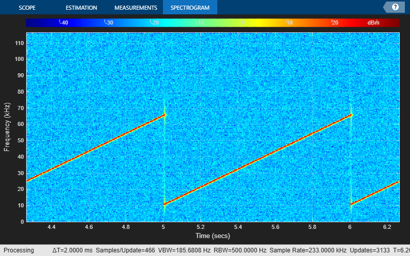
Plot the spectrogram of the noisy chirp signal using the spectrum analyzer. The TimeOrientation property in the spectrum analyzer is set to "vertical". As the simulation time progresses, the spectrogram scrolls in the vertical direction from top to bottom.
Fs = 233e3; frameSize = 20e3; chirp = dsp.Chirp(SampleRate=Fs,SamplesPerFrame=frameSize,... InitialFrequency=11e3,TargetFrequency=11e3+55e3); scope = spectrumAnalyzer(SampleRate=Fs,... AveragingMethod="exponential",... ForgettingFactor=0.3,ViewType="spectrogram",... TimeOrientation="vertical",... RBWSource="property",RBW=500,... TimeSpanSource="property",TimeSpan=2); scope.PlotAsTwoSidedSpectrum = false; for idx = 1:50 y = chirp()+0.05*randn(frameSize,1); scope(y); end

Change the TimeOrientation property to "horizontal". The spectrogram now scrolls in the horizontal direction from right to left.
scope.TimeOrientation = "horizontal"; for idx = 1:50 y = chirp()+0.05*randn(frameSize,1); scope(y); end
Use the Spectrum Analyzer to display frequency input from spectral estimates of sinusoids embedded in white Gaussian noise.
Initialization
Create two dsp.SpectrumEstimator objects. Set one object to use the Welch-based spectral estimation technique with a Hann window. Set the other object to use the filter bank estimation. Specify a noisy sine wave input signal with four sinusoids at 0.16, 0.2, 0.205, and 0.25 cycles per sample. View the spectral estimate using the spectrumAnalyzer object.
FrameSize = 420; Fs = 1; Frequency = [0.16 0.2 0.205 0.25]; sinegen = dsp.SineWave(SampleRate=Fs,SamplesPerFrame=FrameSize,... Frequency=Frequency,Amplitude=[2e-5 1 0.05 0.5]); NoiseVar = 1e-10; numAvgs = 8; hannEstimator = dsp.SpectrumEstimator(PowerUnits="dBm",... Window="Hann",FrequencyRange="onesided",... SpectralAverages=numAvgs,SampleRate=Fs); filterBankEstimator = dsp.SpectrumEstimator(PowerUnits="dBm",... Method="Filter bank",FrequencyRange="onesided",... SpectralAverages=numAvgs,SampleRate=Fs); spectrumPlotter = spectrumAnalyzer(InputDomain="frequency",... SampleRate=Fs,SpectrumUnits="dBm",... YLimits=[-120,40],PlotAsTwoSidedSpectrum=false,... ChannelNames={'Hann window','Filter bank'},ShowLegend=true);
Streaming
Stream the input. Compare the spectral estimates in the spectrum analyzer.
for i = 1:1000 x = sum(sinegen(),2) + sqrt(NoiseVar)*randn(FrameSize,1); Pse_hann = hannEstimator(x); Pfb = filterBankEstimator(x); spectrumPlotter([Pse_hann,Pfb]) end

Compute and display the power spectrum of a noisy sinusoidal input signal using the spectrumAnalyzer object. Measure the peaks, cursor placements, adjacent channel power ratio, and distortion values in the spectrum by enabling these properties:
PeakFinderCursorMeasurementsChannelMeasurementsDistortionMeasurements
Initialization
The input sine wave has two frequencies: 1000 Hz and 5000 Hz. Create two dsp.SineWave System objects to generate these two frequencies. Create a spectrumAnalyzer object to compute and display the power spectrum.
Fs = 44100; Sineobject1 = dsp.SineWave(SamplesPerFrame=1024,PhaseOffset=10,... SampleRate=Fs,Frequency=1000); Sineobject2 = dsp.SineWave(SamplesPerFrame=1024,... SampleRate=Fs,Frequency=5000); SA = spectrumAnalyzer(SampleRate=Fs,SpectrumType="power",... PlotAsTwoSidedSpectrum=false,ChannelNames={'Power spectrum of the input'},... YLimits=[-120 40],ShowLegend=true);
Enable Measurements Data
To obtain the measurements, set the Enabled property to true. Label the peak measurements.
SA.CursorMeasurements.Enabled = true; SA.ChannelMeasurements.Enabled = true; SA.PeakFinder.Enabled = true; SA.PeakFinder.LabelPeaks = true; SA.DistortionMeasurements.Enabled = true;
Use getMeasurementsData
Stream in the noisy sine wave input signal and estimate the power spectrum of the signal using the spectrumAnalyzer object. Measure the characteristics of the spectrum. Use the getMeasurementsData function to obtain these measurements programmatically. The isNewDataReady function returns true when there is new spectrum data. Store the measured data in the variable data.
data = []; for Iter = 1:1000 Sinewave1 = Sineobject1(); Sinewave2 = Sineobject2(); Input = Sinewave1 + Sinewave2; NoisyInput = Input + 0.001*randn(1024,1); SA(NoisyInput); if SA.isNewDataReady data = [data;getMeasurementsData(SA)]; end end

The panels at the bottom of the scope window display the measurements that you have enabled. The values in these panes match the values in the last time step of the data variable. You can access the individual fields of data to obtain the various measurements programmatically.
Compare Peak Values
Use the PeakFinder property to obtain peak values. Verify that the peak values in the last time step of data match the values in the spectrum analyzer plot.
peakvalues = data.PeakFinder(end).Value
peakvalues = 3×1
26.3957
22.7830
-57.9977
frequencieskHz = data.PeakFinder(end).Frequency/1000
frequencieskHz = 3×1
4.9957
0.9905
20.6719
Since R2023b
Use the printToFigure function to print the spectrumAnalyzer object display window to a new MATLAB® figure.
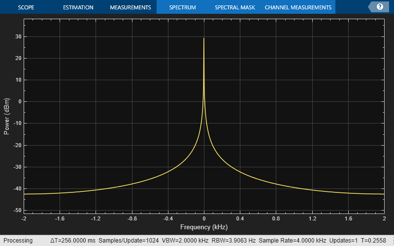
Generate a chirp signal and use the spectrumAnalyzer object to display the spectrum of the chirp. This plot shows the default color and style settings of the spectrumAnalyzer object.
chirp = dsp.Chirp(SweepDirection="Bidirectional", ... TargetFrequency=2000, ... InitialFrequency=0,... TargetTime=400, ... SweepTime=400, ... SamplesPerFrame=1024, ... SampleRate=4000); scope = spectrumAnalyzer(AveragingMethod="exponential",... ForgettingFactor=0,SampleRate=4000); scope(chirp());
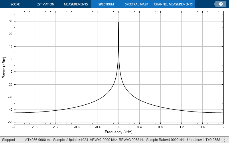
Change the background color and the axes color of the plot to "white". Set the font color and line color to "black".
scope.BackgroundColor = "white"; scope.AxesColor = "white"; scope.FontColor = "black"; scope.LineColor = "black"; show(scope) release(scope)
Print the display of the chirp spectrum to a new MATLAB figure. The function returns a handle to the figure.
scopeFig = printToFigure(scope);

The handle to the figure scopeFig lets you modify the appearance and the behavior of the figure window.
Specify a figure name and change the size of the figure to 400-by-250 pixels.
scopeFig.Name="Spectrum of Chirp Signal"; scopeFig.NumberTitle="off"; scopeFig.Position=[1 1 400 250];
When printing to figure, you can make the figure invisible by setting the Visible argument to false.
scopeFig = printToFigure(scope,Visible=false);
Limitations
Does not support C/C++ code generation using MATLAB Coder™. To generate a standalone application, use the MATLAB Compiler™.
Supports MEX code generation by treating the calls to the object as extrinsic.
More About
Measure harmonic distortion and intermodulation distortion.
When you click the Distortion button in the Distortion section of the Measurements tab, a distortion panel opens at the bottom of the Spectrum Analyzer window. This panel shows the harmonic and distortion measurement values for the input signal currently on display in the scope. The Distortion section in the Measurements tab allows you to specify the distortion type, number of harmonics, and even label the harmonics.
Note
For an accurate measurement, ensure that the fundamental signal (for harmonics) or
primary tones (for intermodulation) is larger than any spurious or harmonic content. To
do so, you may need to adjust the resolution bandwidth (RBW) of the
Spectrum Analyzer. Make sure that the bandwidth is low enough to isolate the signal and
harmonics from spurious noise content. In general, you should set the RBW value such
that there is at least a 10 dB separation between the peaks of the sinusoids and the
noise floor. You also might need to select a different spectral window to obtain a valid
measurement.
You can set the Distortion Type parameter to one of these values:
Harmonic–– SelectHarmonicif your input is a single sinusoid.Intermodulation–– SelectIntermodulationif your input is two equal-amplitude sinusoids. Intermodulation can help you determine distortion when the scope uses only a small portion of the available bandwidth.
See Distortion Measurements for information on how distortion measurements are calculated.
When you set the Distortion Type to Harmonic,
these fields appear in the Harmonic Distortion panel at the bottom
of the Spectrum Analyzer window.
H1 — Fundamental frequency in Hz and its power in decibels of the measured power referenced to 1 milliwatt (dBm).
H2, H3, ... — Harmonics frequencies in Hz and their power in decibels relative to the carrier (dBc). If the harmonics are at the same level or exceed the fundamental frequency, reduce the input power.
THD — Total harmonic distortion. This value represents the ratio of the power in the harmonics D to the power in the fundamental frequency S. If the noise power is too high in relation to the harmonics, the THD value is not accurate. In this case, lower the resolution bandwidth or select a different spectral window.
SNR — Signal-to-noise ratio (SNR). This value represents the ratio of the power in the fundamental frequency S to the power of all nonharmonic content N, including spurious signals, in decibels relative to the carrier (dBc).
If you see
––as the reported SNR, the total nonharmonic content of your signal is less than 30% of the total signal.SINAD — Signal-to-noise-and-distortion ratio. This value represents the ratio of the power in the fundamental frequency S to all other content (including noise N and harmonic distortion D) in decibels relative to the carrier (dBc).
SFDR — Spurious-free dynamic range (SFDR). This value represents the ratio of the power in the fundamental frequency S to power of the largest spurious signal R regardless of where it falls in the frequency spectrum. The worst spurious signal might or might not be a harmonic of the original signal. SFDR represents the smallest value of a signal that can be distinguished from a large interfering signal. SFDR includes harmonics.
The harmonic distortion measurement automatically locates the largest sinusoidal component (fundamental signal frequency). It then computes the harmonic frequencies and power in each harmonic in your signal and ignores any DC component. The measurement does not include any harmonics that are outside the Spectrum Analyzer frequency span. Adjust your frequency span so that it includes all the desired harmonics.
Note
To view the best harmonics, make sure that your fundamental frequency is set high enough to resolve the harmonics. However, this frequency should not be so high that aliasing occurs. For the best display of harmonic distortion, your plot should not show skirts, which indicate frequency leakage. The noise floor should be visible.
For a better display, try a Kaiser window with a large sidelobe attenuation (e.g. between 100–300 db).


When you set the Distortion Type to
Intermodulation, the following fields appear in the
Intermodulation Distortion panel at the bottom of the Spectrum
Analyzer window.
F1 — Lower fundamental first-order frequency.
F2 — Upper fundamental first-order frequency.
2F1 - F2 — Lower intermodulation product from third-order harmonics.
2F2 - F1 — Upper intermodulation product from third-order harmonics.
TOI — Third-order intercept point. If the noise power is too high in relation to the harmonics, the TOI value will not be accurate. In this case, you should lower the resolution bandwidth or select a different spectral window. If the TOI has the same amplitude as the input two-tone signal, reduce the power of that input signal.
The intermodulation distortion measurement automatically locates the fundamental and the first-order frequencies (F1 and F2). It then computes the frequencies of the third-order intermodulation products (2F1−F2 and 2F2−F1).
For modifying the distortion measurements programmatically, see the DistortionMeasurementsConfiguration object. For more information on these
settings in the UI, see Distortion.
Set configuration and style settings in the Spectrum Analyzer.
To control the settings of the display and labels, color and styling, click on
Settings (![]() ) in the Scope tab of the Spectrum
Analyzer toolstrip.
) in the Scope tab of the Spectrum
Analyzer toolstrip.
In the dialog box that opens, you can customize the font size, plot type, y-axis properties of the spectrum plot, and color map properties of the spectrogram plot. You can change the color of the spectrum plot, background, axes, and labels and also change the line properties.
When you view the spectrum or the spectrogram, you see only the relevant options. For more details about these options, see Configuration > Spectrum Settings.
Zoom and pan axes using display controls.
To scale the plot axes, use the mouse to pan around the axes and the scroll button on your mouse to zoom in and out of the plot. Additionally, you can use the buttons that appear when you hover over the plot window.
 — Maximize the axes, hide all labels and inset
the axes values.
— Maximize the axes, hide all labels and inset
the axes values. — Zoom in on the plot.
 — Pan the plot.
 — Autoscale the axes to fit the shown data.
Tips
To close the scope window and clear its associated data, use the MATLAB
clearfunction.To hide or show the scope window, use the
hideandshowfunctions.Use the MATLAB
mccfunction to compile code containing a Spectrum Analyzer.If you set the
AveragingMethodto"vbw"or"exponential", and you introduceNaNorInfvalues into the data, the spectrum appears blank. To configure the spectrum analyzer to ignoreNaNorInfvalues, on the Home tab in the MATLAB toolstrip, in the Environment section, click Settings ( ). In the Workspace section of the
Settings dialog box, select the Ignore NaNs when
calculating statistics check box.
). In the Workspace section of the
Settings dialog box, select the Ignore NaNs when
calculating statistics check box.
Algorithms
When you choose the Filter Bank method, the spectrum
analyzer uses an analysis filter bank to estimate the power spectrum.
The filter bank splits the broadband input signal x(n), of sample rate fs, into multiple narrow band signals y0(m), y1(m), … , yM-1(m), of sample rate fs/M.
The variable M represents the number of frequency bands in the
filter bank. In the spectrum analyzer, M is equal to the number of
data points needed to achieve the specified RBW value or 1024, whichever is larger. For
more information on the analysis filter bank and its implementation, see the More About and the Algorithm sections in the
dsp.Channelizer object.
After the spectrum analyzer splits the broadband input signal into multiple narrow bands, it computes the power in each narrow frequency band using the following equation. Each Zi value is the power estimate over that narrow frequency band.
L is length of the narrowband signal yi(m) and i = 1, 2, …, M−1.
The power values in all the narrow frequency bands (denoted by Zi) form the Z vector.
The spectrum analyzer averages the current Z vector with the previous Z vectors using one of the moving average methods: video bandwidth, exponential weighting, or running. The output of the averaging operation forms the spectral estimate vector. For details on the two averaging methods, see Averaging Method.

The spectrum analyzer uses the value you specify in the RBW (Hz) parameter or the Number of frequency bands parameter to determine the input frame length.
When you specify the Resolution Method to
RBW, and you set RBW (Hz) to:
Auto–– The spectrum analyzer determines the appropriate resolution bandwidth to ensure that there are 1024 RBW intervals over the specified frequency span. When you set RBW (Hz) toAuto, the spectrum analyzer calculates RBW using this equation.scalar value –– The spectrum analyzer calculates the number of samples Nsamples using this equation.
Fs is the sample rate of the input signal as specified in the Sample Rate (Hz) property.
The RBW value you specify must be such that there are at least two RBW intervals over the specified frequency span. The ratio of the overall span to RBW must be greater than two.
span is the frequency span over which the spectrum analyzer computes and plots the spectrum. To view the Span (Hz) in the scope, click the Estimation tab on the spectrum analyzer toolstrip and navigate to the Frequency Options section. To enable this property, set Frequency Span to
Span and Center Frequency.
When you specify the Resolution Method to Number of
frequency bands, the resulting RBW is given by:
When the number of input samples is not sufficient to achieve the specified resolution bandwidth, the spectrum analyzer adjusts its RBW value according to the number of input samples provided and displays a message similar to this one. The spectrum analyzer removes this message once you provide enough input samples.

Fs is the sample rate of the input signal.
To view the Sample Rate (Hz) in the scope, click the
Scope tab on the spectrum analyzer toolstrip and navigate to
the Bandwidth section. You can enable this property in the status
bar at the bottom of the spectrum analyzer window. Click the ![]() icon in the status bar and select
icon in the status bar and select Sample
Rate.
Resolution bandwidth controls the spectral resolution of the displayed signal. The RBW value determines the spacing between frequencies that the scope can resolve. A smaller value gives a higher spectral resolution and lowers the noise floor, that is, the spectrum analyzer can resolve frequencies that are closer to each other. However, this comes at the cost of a longer sweep time.
You can specify the resolution bandwidth using the RBW (Hz) parameter.
If you specify the window length, the scope determines the RBW value from the window length using this equation, .
When you specify the Resolution
Method to RBW, and you set RBW
(Hz) to:
Auto–– The spectrum analyzer determines the appropriate resolution bandwidth to ensure that there are 1024 RBW intervals over the specified frequency span. When you set RBW (Hz) toAuto, the spectrum analyzer calculates using this equation.scalar value –– Specify a value such that there are at least two RBW intervals over the specified frequency span. The ratio of the overall span to RBW must be greater than two:
span is the frequency span over which the spectrum analyzer
computes and plots the spectrum. Spectrum analyzer shows the span through the
Span (Hz) property. To view the Span (Hz)
in the scope, click the Estimation tab on the spectrum analyzer
toolstrip, navigate to the Frequency Options section, and set
Frequency Span to Span and Center
Frequency.
When you specify the Resolution
Method to Number of frequency bands, the
resulting RBW is given by:
When the number of input samples is not sufficient to achieve the specified resolution bandwidth, the spectrum analyzer adjusts its RBW value according to the number of input samples provided and displays a message similar to this one. The spectrum analyzer removes this message once you provide enough input samples.
You can enable this property in the status bar at the bottom of the spectrum analyzer
window. Click the ![]() icon in the status bar and select
icon in the status bar and select
RBW.