fgls

Feasible generalized least squares

Syntax

[coeff,se,EstCoeffCov] = fgls(X,y)

[CoeffTbl,CovTbl] = fgls(Tbl)

[___] = fgls(___,Name=Value)

[___] = fgls(ax,___,Plot=plot)

[___,iterPlots] = fgls(___,Plot=plot)

Description

[coeff,se,EstCoeffCov] = fgls(X,y) returns vectors of coefficient estimates and corresponding standard errors, and the estimated coefficient covariance matrix, from applying feasible generalized least squares (FGLS) to the multiple linear regression model y = Xβ + ε. y is a vector of response data and X is a matrix of predictor data.

[CoeffTbl,CovTbl] = fgls(Tbl) returns a table containing FGLS coefficient estimates and corresponding standard errors, and a table containing the FGLS estimated coefficient covariance matrix, from applying FGLS to the variables in the input table or timetable. The response variable in the regression is the last variable, and all other variables are the predictor variables.

To select a different response variable for the regression, use the ResponseVariable name-value argument. To select different predictor variables, use the PredictorNames name-value argument.

[___] = fgls(___,Name=Value) specifies options using one or more name-value arguments in addition to any of the input argument combinations in previous syntaxes. fgls returns the output argument combination for the corresponding input arguments.

For example, fgls(Tbl,ResponseVariable="GDP",InnovMdl="H4",Plot="all") provides coefficient, standard error, and residual mean-squared error (MSE) plots of iterations of FGLS for a regression model with White’s robust innovations covariance, and the table variable GDP is the response while all other variables are predictors.

[___] = fgls(ax,___,Plot=plot) plots on the axes specified in ax instead of the axes of new figures when plot is not "off". ax can precede any of the input argument combinations in the previous syntaxes.

[___,iterPlots] = fgls(___,Plot=plot) returns handles to plotted graphics objects when plot is not "off". Use elements of iterPlots to modify properties of the plots after you create them.

Examples

Estimate FGLS Coefficients and Uncertainty Measures

Suppose the sensitivity of the US consumer price index (CPI) to changes in the paid compensation of employees (COE) is of interest.

Load the US macroeconomic data set, which contains the timetable of data DataTimeTable. Extract the COE and CPI series from the table.

load Data_USEconModel.mat
COE = DataTimeTable.COE;
CPI = DataTimeTable.CPIAUCSL;
dt = DataTimeTable.Time;

Plot the series.

tiledlayout(2,1)
nexttile
plot(dt,CPI);
title("\bf Consumer Price Index, Q1 in 1947 to Q1 in 2009");
axis tight
nexttile
plot(dt,COE);
title("\bf Compensation Paid to Employees, Q1 in 1947 to Q1 in 2009");
axis tight

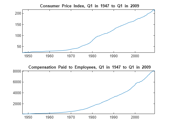
The series are nonstationary. Stabilize them by computing their returns.

rCPI = price2ret(CPI);
rCOE = price2ret(COE);

Regress rCPI onto rCOE including an intercept to obtain ordinary least squares (OLS) estimates, standard errors, and the estimated coefficient covariance. Generate a lagged residual plot.

Mdl = fitlm(rCOE,rCPI);
clmCoeff = Mdl.Coefficients.Estimate

clmCoeff = 2×1

    0.0033
    0.3513

clmSE = Mdl.Coefficients.SE

clmSE = 2×1

    0.0010
    0.0490

CLMEstCoeffCov = Mdl.CoefficientCovariance

CLMEstCoeffCov = 2×2

    0.0000   -0.0000
   -0.0000    0.0024

figure
plotResiduals(Mdl,"lagged")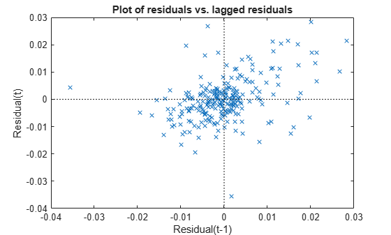

The residual plot exhibits an upward trend, which suggests that the innovations comprise an autoregressive process. This violates one of the classical linear model assumptions. Consequently, hypothesis tests based on the regression coefficients are incorrect, even asymptotically.

Estimate the regression coefficients, standard errors, and coefficient covariances using FGLS. By default, fgls includes an intercept in the regression model and imposes an AR(1) model on the innovations.

[coeff,se,EstCoeffCov] = fgls(rCPI,rCOE)

coeff = 2×1

    0.0148
    0.1961

se = 2×1

    0.0012
    0.0685

EstCoeffCov = 2×2

    0.0000   -0.0000
   -0.0000    0.0047

Row 1 of the outputs corresponds to the intercept and row 2 corresponds to the coefficient of rCOE.

If the COE series is exogenous with respect to the CPI, then the FGLS estimates coeff are consistent and asymptotically more efficient than the OLS estimates.

Estimate FGLS Coefficients and Uncertainty Measures on Table Data

Load the US macroeconomic data set, which contains the timetable of data DataTimeTable.

load Data_USEconModel

Stabilize all series by computing their returns.

RDT = price2ret(DataTimeTable);

RDT is a timetable of returns of all variables in DataTimeTable. The price2ret function conserves variable names.

Estimate the regression coefficients, standard errors, and the coefficient covariance matrix using FGLS. Specify the response and predictor variable names.

[CoeffTbl,CoeffCovTbl] = fgls(RDT,ResponseVariable="CPIAUCSL",PredictorVariables="COE")

CoeffTbl=2×2 table
               Coeff          SE    
             __________    _________

    Const    6.2416e-05    1.336e-05
    COE         0.20562     0.055615

CoeffCovTbl=2×2 table
                Const           COE    
             ___________    ___________

    Const     1.7848e-10    -5.6329e-07
    COE      -5.6329e-07       0.003093

When you supply a table or timetable of data, fgls returns tables of estimates.

Specify AR Lags For FGLS Estimation

Suppose the sensitivity of the US consumer price index (CPI) to changes in the paid compensation of employees (COE) is of interest. This example expands on the analysis outlined in the example Estimate FGLS Coefficients and Uncertainty Measures.

Load the US macroeconomic data set.

load Data_USEconModel

The series are nonstationary. Stabilize them by applying the log, and then the first difference.

LDT = price2ret(Data);
rCOE = LDT(:,1);
rCPI = LDT(:,2);

Regress rCPI onto rCOE, which includes an intercept to obtain OLS estimates. Plot correlograms for the residuals.

Mdl = fitlm(rCOE,rCPI);
u = Mdl.Residuals.Raw;

figure;
subplot(2,1,1)
autocorr(u);
subplot(2,1,2);
parcorr(u);

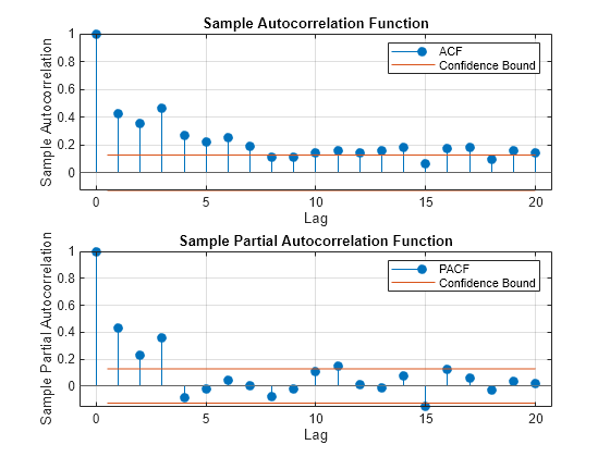
The correlograms suggest that the innovations have significant AR effects. According to Box-Jenkins methodology, the innovations seem to comprise an AR(3) series. For details, see Select ARIMA Model for Time Series Using Box-Jenkins Methodology.

Estimate the regression coefficients using FGLS. By default, fgls assumes that the innovations are autoregressive. Specify that the innovations are AR(3) by using the ARLags name-value argument, and print the final estimates to the command window by using the Display name-value argument.

fgls(rCPI,rCOE,ARLags=3,Display="final");

OLS Estimates:

       |  Coeff    SE   
------------------------
 Const | 0.0122  0.0009 
 x1    | 0.4915  0.0686 

FGLS Estimates:

       |  Coeff    SE   
------------------------
 Const | 0.0148  0.0012 
 x1    | 0.1972  0.0684 

If the COE rate series is exogenous with respect to the CPI rate, the FGLS estimates are consistent and asymptotically more efficient than the OLS estimates.

Account for Residual Heteroscedasticity Using FGLS Estimation

Model the nominal GNP GNPN growth rate accounting for the effects of the growth rates of the consumer price index CPI, real wages WR, and the money stock MS. Account for classical linear model departures.

Load the Nelson-Plosser data set, which contains the data in the table DataTable. Remove all observations containing at least one missing value.

load Data_NelsonPlosser
DT = rmmissing(DataTable);
T = height(DT);                       

Plot the series.

predNames = ["CPI" "WR" "MS"];

tiledlayout(2,2)
for j = ["GNPN" predNames]
    nexttile
    plot(DT{:,j});
    xticklabels(DT.Dates)
    title(j);
    axis tight
end

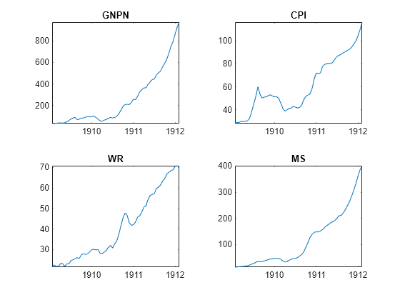
All series appear nonstationary.

For each series, compute the returns.

RetDT = price2ret(DT);

RetTT is a timetable of the returns of the variables in TT. The variables names are conserved.

Regress the GNPN rate onto the CPI, WR, and MS rates. Examine a scatter plot and correlograms of the residuals.

Mdl = fitlm(RetDT,ResponseVar="GNPN",PredictorVar=predNames);

figure
plotResiduals(Mdl,"caseorder");
axis tight

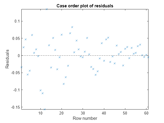
figure
tiledlayout(2,1)
nexttile
autocorr(Mdl.Residuals.Raw);
nexttile
parcorr(Mdl.Residuals.Raw);

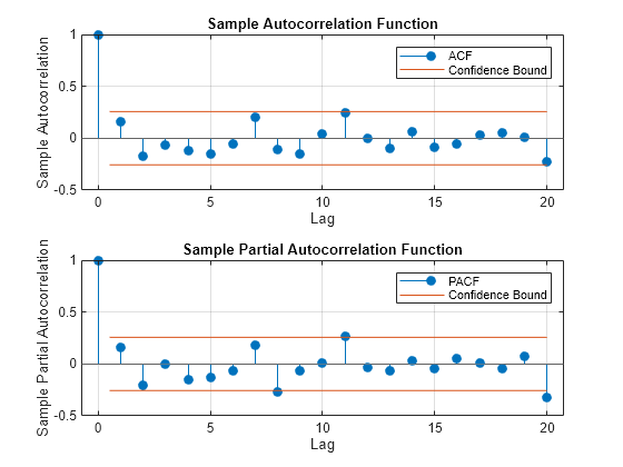
The residuals appear to flare in, which is indicative of heteroscedasticity. The correlograms suggest that there is no autocorrelation.

Estimate FGLS coefficients by accounting for the heteroscedasticity of the residuals. Specify that the estimated innovation covariance is diagonal with the squared residuals as weights (that is, White's robust estimator H0).

fgls(RetDT,ResponseVariable="GNPN",PredictorVariables=predNames, ...
    InnovMdl="HC0",Display="final");

OLS Estimates:

       |  Coeff     SE   
-------------------------
 Const | -0.0076  0.0085 
 CPI   |  0.9037  0.1544 
 WR    |  0.9036  0.1906 
 MS    |  0.4285  0.1379 

FGLS Estimates:

       |  Coeff     SE   
-------------------------
 Const | -0.0102  0.0017 
 CPI   |  0.8853  0.0169 
 WR    |  0.8897  0.0294 
 MS    |  0.4874  0.0291 

Estimate FGLS Coefficients of Models Containing ARMA Errors

Create this regression model with ARMA(1,2) errors, where $${\epsilon }_t$$ is Gaussian with mean 0 and variance 1.

$$\begin{array}{c}{y}_t=1+x_t\left[\begin{array}{c}2\\ 3\end{array}\right]+u_t\\ u_t=0.6u_{t-1}+{\epsilon }_t-0.3{\epsilon }_{t-1}+0.1{\epsilon }_{t-1}.\end{array}$$

beta = [2 3];
phi = 0.2;
theta = [-0.3 0.1];
Mdl = regARIMA(AR=phi,MA=theta,Intercept=1, ...
    Beta=beta,Variance=1);

Mdl is a regARIMA model. You can access its properties using dot notation.

Simulate 500 periods of 2-D standard Gaussian values for $$x_t$$, and then simulate responses using Mdl.

numObs = 500;
rng(1); % For reproducibility
X = randn(numObs,2);
y = simulate(Mdl,numObs,X=X);

fgls supports AR(p) innovation models. You can convert an ARMA model polynomial to an infinite-lag AR model polynomial using arma2ar. By default, arma2ar returns the coefficients for the first 10 terms. After the conversion, determine how many lags of the resulting AR model are practically significant by checking the length of the returned vector of coefficients. Choose the number of terms that exceed 0.00001.

format long
arParams = arma2ar(phi,theta)

arParams = 1×3

  -0.100000000000000   0.070000000000000   0.031000000000000

arLags = sum(abs(arParams) > 0.00001);
format short

Some of the parameters have small magnitude. You might want to reduce the number of lags to include in the innovations model for fgls.

Estimate the coefficients and their standard errors using FGLS and the simulated data. Specify that the innovations comprise an AR(arLags) process.

[coeff,~,EstCoeffCov] = fgls(X,y,InnovMdl="AR",ARLags=arLags)

coeff = 3×1

    1.0372
    2.0366
    2.9918

EstCoeffCov = 3×3

    0.0026   -0.0000    0.0001
   -0.0000    0.0022    0.0000
    0.0001    0.0000    0.0024

The estimated coefficients are close to their true values.

Plot Iterations of FGLS Estimation

This example expands on the analysis in Estimate FGLS Coefficients of Models Containing ARMA Errors. Create this regression model with ARMA(1,4) errors, where $${\epsilon }_t$$ is Gaussian with mean 0 and variance 1.

$$\begin{array}{c}{y}_t=1+x_t\left[\begin{array}{c}1.5\\ 2\end{array}\right]+u_t\\ u_t=0.9u_{t-1}+{\epsilon }_t-0.4{\epsilon }_{t-1}+0.2{\epsilon }_{t-4}.\end{array}$$

beta = [1.5 2];
phi = 0.9;
theta = [-0.4 0.2];
Mdl = regARIMA(AR=phi,MA=theta,MALags=[1 4],Intercept=1,Beta=beta,Variance=1);

Suppose the distribution of the predictors is

$$x_t\sim N\left(\left[\begin{array}{c}-1\\ 1\end{array}\right],\left[\begin{array}{cc}0.25& 0\\ 0& 1\end{array}\right]\right).$$

Simulate 30 periods from ${\mathit{x}}_{\mathit{t}}$, and then simulate 30 corresponding responses from the regression model with ARMA errors Mdl.

numObs = 30;
rng(1); % For reproducibility
muX = [-1 1];
sigX = [0.5 1];
X = randn(numObs,numel(beta)).*sigX + muX;
y = simulate(Mdl,numObs,X=X);

Convert the ARMA model polynomial to an infinite-lag AR model polynomial using arma2ar. By default, arma2ar returns the coefficients for the first 10 terms. Find the number of terms that exceed 0.00001.

arParams = arma2ar(phi,theta);
arLags = sum(abs(arParams) > 1e-5);

Estimate the regression coefficients by using eight iterations of FGLS, and specify the number of lags in the AR innovation model (arLags). Also, specify to plot the coefficient estimates and their standard errors for each iteration, and to display the final estimates and the OLS estimates in tabular form.

[coeff,~,EstCoeffCov] = fgls(X,y,InnovMdl="AR",ARLags=arLags, ...
    NumIter=8,Plot=["coeff" "se"],Display="final");

OLS Estimates:

       |  Coeff    SE   
------------------------
 Const | 1.7619  0.4514 
 x1    | 1.9637  0.3480 
 x2    | 1.7242  0.2152 

FGLS Estimates:

       |  Coeff    SE   
------------------------
 Const | 1.0845  0.6972 
 x1    | 1.7020  0.2919 
 x2    | 2.0825  0.1603 

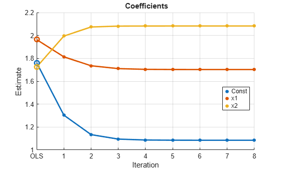
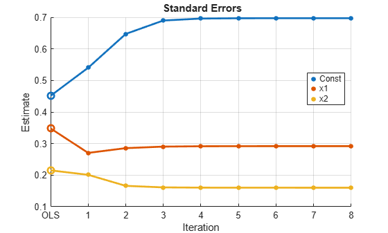
The algorithm seems to converge after the four iterations. The FGLS estimates are closer to the true values than the OLS estimates.

Properties of iterative FGLS estimates in finite samples are difficult to establish. For asymptotic properties, one iteration of FGLS is sufficient, but fgls supports iterative FGLS for experimentation.

If the estimates or standard errors show instability after successive iterations, then the estimated innovations covariance might be ill conditioned. Consider scaling the residuals by using the ResCond name-value argument to improve the conditioning of the estimated innovations covariance.

Input Arguments

X — Predictor data X

numeric matrix

Predictor data X for the multiple linear regression model, specified as a numObs-by-numPreds numeric matrix.

Each row represents one of the numObs observations and each column represents one of the numPreds predictor variables.

Data Types: double

y — Response data y

numeric vector

Response data y for the multiple linear regression model, specified as a numObs-by-1 numeric vector. Rows of y and X correspond.

Data Types: double

Tbl — Combined predictor and response data

table | timetable

Combined predictor and response data for the multiple linear regression model, specified as a table or timetable with numObs rows. Each row of Tbl is an observation.

The test regresses the response variable, which is the last variable in Tbl, on the predictor variables, which are all other variables in Tbl. To select a different response variable for the regression, use the ResponseVariable name-value argument. To select different predictor variables, use the PredictorNames name-value argument to select numPreds predictors.

ax — Axes on which to plot

vector of Axes objects

Axes on which to plot, specified as a vector of Axes objects with length equal to the number of plots specified by the Plot name-value argument.

By default, fgls creates a separate figure for each plot.

Note

NaNs in X, y, or Tbl indicate missing values, and fgls removes observations containing at least one NaN. That is, to remove NaNs in X or y, fgls merges the variables [X y], and then it uses list-wise deletion to remove any row that contains at least one NaN. fgls also removes any row of Tbl containing at least one NaN. Removing NaNs in the data reduces the sample size and can create irregular time series.

Name-Value Arguments

Specify optional pairs of arguments as Name1=Value1,...,NameN=ValueN, where Name is the argument name and Value is the corresponding value. Name-value arguments must appear after other arguments, but the order of the pairs does not matter.

Before R2021a, use commas to separate each name and value, and enclose Name in quotes.

Example: fgls(Tbl,ResponseVariable="GDP",InnovMdl="H4",Plot="all") provides coefficient, standard error, and residual mean squared error (RMSE) plots of iterations of FGLS for a regression model with White’s robust innovations covariance, and the table variable GDP is the response while all other variables are predictors.

VarNames — Unique variable names to use in display

string vector | character vector | cell vector of strings | cell vector of character vectors

Unique variable names used in the display, specified as a string vector or cell vector of strings of a length numCoeffs:

• If Intercept=true, VarNames(1) is the name of the intercept (for example 'Const') and VarNames(j + 1) specifies the name to use for variable X(:,j) or PredictorVariables(j).

• If Intercept=false, VarNames(j) specifies the name to use for variable X(:,j) or PredictorVariables(j).

The defaults is one of the following alternatives prepended by 'Const' when an intercept is present in the model:

• {'x1','x2',...} when you supply inputs X and y

• Tbl.Properties.VariableNames when you supply input table or timetable Tbl

Example: VarNames=["Const" "AGE" "BBD"]

Data Types: char | cell | string

Intercept — Flag to include intercept

true (default) | false

Flag to include a model intercept, specified as a value in this table.

Value	Description
true	fgls includes an intercept term in the regression model. numCoeffs = numPreds + 1.
false	fgls does not include an intercept when fitting the regression model. numCoeffs = numPreds.

Example: Intercept=false

Data Types: logical

InnovMdl — Model for innovations covariance estimate

"AR" (default) | "CLM" | "HC0" | "HC1" | "HC2" | "HC3" | "HC4" | character vector

Model for the innovations covariance estimate, specified as a model name in the following table.

Set InnovMdl to specify the structure of the innovations covariance estimator $$\widehat{\Omega }$$.

• For diagonal innovations covariance models (i.e., models with heteroscedasticity), $$\widehat{\Omega }=diag(\omega ),$$ where ω = {ω_i; i = 1,...,T} is a vector of innovation variance estimates for the observations, and T = numObs.

  fgls estimates the data-driven vector ω using the corresponding model residuals (ε), their leverages $$h_i=x_i{(X^{\prime }X)}^{-1}{x}_i^{\prime },$$ and the degrees of freedom dfe.

  Model Name	Weight	Reference
  "CLM"	$${\omega }_i=\frac{1}{dfe}{\displaystyle \sum }_{i=1}^T{\epsilon }_i^2$$	[4]
  "HC0"	$${\omega }_i={\epsilon }_i^2$$	[6]
  "HC1"	$${\omega }_i=\frac{T}{dfe}{\epsilon }_i^2$$	[5]
  "HC2"	$${\omega }_i=\frac{{\epsilon }_i^2}{1-h_i}$$	[5]
  "HC3"	$${\omega }_i=\frac{{\epsilon }_i^2}{{(1-h_i)}^2}$$	[5]
  "HC4"	$${\omega }_i=\frac{{\epsilon }_i^2}{{(1-h_i)}^{d_i}}$$ where $$d_i=\min \left(4,\frac{h_i}{\overline{h}}\right)$$	[1]

• For full innovation covariance models (in other words, models having heteroscedasticity and autocorrelation), specify "AR". fgls imposes an AR(p) model on the innovations, and constructs $$\widehat{\Omega }$$ using the number of lags, p, specified by the name-value argument arLags and the Yule-Walker equations.

If the NumIter name-value argument is 1 and you specify the InnovCov0 name-value argument, fgls ignores InnovMdl.

Example: InnovMdl=HC0

Data Types: char | string

ARLags — Number of lags

1 (default) | positive integer

Number of lags to include in the autoregressive (AR) innovations model, specified as a positive integer.

If the InnovMdl name-value argument is not "AR" (that is, for diagonal models), fgls ignores ARLags.

For general ARMA innovations models, convert the innovations model to the equivalent AR form by performing one of the following actions.

• Construct the ARMA innovations model lag operator polynomial using LagOp. Then, divide the AR polynomial by the MA polynomial using, for example, mrdivide. The result is the infinite-order, AR representation of the ARMA model.

• Use arma2ar, which returns the coefficients of the infinite-order, AR representation of the ARMA model.

Example: ARLags=4

Data Types: double

InnovCov0 — Initial innovations covariance

[] (default) | positive vector | positive definite matrix | positive semidefinite matrix

Initial innovations covariance, specified as a positive vector, positive semidefinite matrix, or a positive definite matrix.

InnovCov0 replaces the data-driven estimate of the innovations covariance ($$\widehat{\Omega }$$) in the first iteration of GLS.

• For diagonal innovations covariance models (that is, models with heteroscedasticity), specify a numObs-by-1 vector. InnovCov0(j) is the variance of innovation j.

• For full innovation covariance models (that is, models having heteroscedasticity and autocorrelation), specify a numObs-by-numObs matrix. InnovCov0(j,k) is the covariance of innovations j and k.

By default, fgls uses a data-driven $$\widehat{\Omega }$$ (see the InnovMdl name-value argument).

Data Types: double

NumIter — Number of iterations

1 (default) | positive integer

Number of iterations to implement for the FGLS algorithm, specified as a positive integer.

fgls estimates the innovations covariance $$\widehat{\Omega }$$ at each iteration from the residual series according to the innovations covariance model InnovMdl. Then, the software computes the GLS estimates of the model coefficients.

Example: NumIter=10

Data Types: double

ResCond — Flag to scale residuals

false (default) | true

Flag to scale the residuals at each iteration of FGLS, specified as a value in this table.

Value	Description
true	fgls scales the residuals at each iteration.
false	fgls does not scale the residuals at each iteration.

Tip

The setting ResCond=true can improve the conditioning of the estimation of the innovations covariance $$\widehat{\Omega }$$.

Data Types: logical

Display — Command window display control

"off" (default) | "final" | "iter" | character vector

Command window display control, specified as a value in this table.

Value	Description
"final"	fgls displays the final estimates.
"iter"	fgls displays the estimates after each iteration.
"off"	fgls suppresses command window display.

fgls shows estimation results in tabular form.

Example: Display="iter"

Data Types: char | string

Plot — Control for plotting results

"off" (default) | "all" | "coeff" | "mse" | "se" | character vector | string vector | cell array of character vectors

Control for plotting results after each iteration, specified as a value in the following table, or a string vector or cell array of character vectors of such values.

To examine the convergence of the FGLS algorithm, specify plotting the estimates for each iteration.

Value	Description
"all"	fgls plots the estimated coefficients, their standard errors, and the residual mean-squared error (MSE) on separate plots.
"coeff"	fgls plots the estimated coefficients.
"mse"	fgls plots the MSEs.
"off"	fgls does not plot the results.
"se"	fgls plots the estimated coefficient standard errors.

Example: Plot="all"

Example: Plot=["coeff" "se"] separately plots iterative coefficient estimates and their standard errors.

Data Types: char | string | cell

ResponseVariable — Variable in Tbl to use for response

first variable in Tbl (default) | string vector | cell vector of character vectors | vector of integers | logical vector

Variable in Tbl to use for response, specified as a string vector or cell vector of character vectors containing variable names in Tbl.Properties.VariableNames, or an integer or logical vector representing the indices of names. The selected variables must be numeric.

fgls uses the same specified response variable for all tests.

Example: ResponseVariable="GDP"

Example: ResponseVariable=[true false false false] or ResponseVariable=1 selects the first table variable as the response.

Data Types: double | logical | char | cell | string

PredictorVariables — Variables in Tbl to use for the predictors

string vector | cell vector of character vectors | vector of integers | logical vector

Variables in Tbl to use for the predictors, specified as a string vector or cell vector of character vectors containing variable names in Tbl.Properties.VariableNames, or an integer or logical vector representing the indices of names. The selected variables must be numeric.

fgls uses the same specified predictors for all tests.

By default, fgls uses all variables in Tbl that are not specified by the ResponseVariable name-value argument.

Example: PredictorVariables=["UN" "CPI"]

Example: PredictorVariables=[false true true false] or DataVariables=[2 3] selects the second and third table variables.

Data Types: double | logical | char | cell | string

Output Arguments

coeff — FGLS coefficient estimates

numeric vector

FGLS coefficient estimates, returned as a numCoeffs-by-1 numeric vector. fgls returns coeff when you supply the inputs X and y.

Rows of coeff correspond to the predictor matrix columns, with the first row corresponding to the intercept when Intercept=true. For example, in a model with an intercept, the value of $${\widehat{\beta }}_1$$ (corresponding to the predictor x₁) is in position 2 of coeff.

se — Coefficient standard error estimates

numeric vector

Coefficient standard error estimates, returned as a numCoeffs-by-1 numeric. The elements of se are sqrt(diag(EstCoeffCov)). fgls returns se when you supply the inputs X and y.

Rows of se correspond to the predictor matrix columns, with the first row corresponding to the intercept when Intercept=true. For example, in a model with an intercept, the estimated standard error of $${\widehat{\beta }}_1$$ (corresponding to the predictor x₁) is in position 2 of se, and is the square root of the value in position (2,2) of EstCoeffCov.

EstCoeffCov — Coefficient covariance matrix estimate

numeric matrix

Coefficient covariance matrix estimate, returned as a numCoeffs-by-numCoeffs numeric matrix. fgls returns EstCoeffCov when you supply the inputs X and y.

Rows and columns of EstCoeffCov correspond to the predictor matrix columns, with the first row and column corresponding to the intercept when Intercept=true. For example, in a model with an intercept, the estimated covariance of $${\widehat{\beta }}_1$$ (corresponding to the predictor x₁) and $${\widehat{\beta }}_2$$ (corresponding to the predictor x₂) are in positions (2,3) and (3,2) of EstCoeffCov, respectively.

CoeffTbl — FGLS coefficient estimates and standard errors

table

FGLS coefficient estimates and standard errors, returned as a numCoeffs-by-2 table. fgls returns CoeffTbl when you supply the input Tbl.

For j = 1,…,numCoeffs, row j of CoeffTbl contains estimates of coefficient j in the regression model and it has label VarNames(j). The first variable Coeff contains the coefficient estimates coeff and the second variable SE contains the standard errors se.

CovTbl — Coefficient covariance matrix estimate

table

Coefficient covariance matrix estimate, returned as a numCoeffs-by-numCoeffs table containing the coefficient covariance matrix estimate EstCoeffCov. fgls returns CovTbl when you supply the input Tbl.

For each pair (i,j), CovTbl(i,j) contains the covariance estimate of coefficients i and j in the regression model. The label of row and variable j is VarNames(j), j = 1,…,numCoeffs.

iterPlots — Handles to plotted graphics objects

structure array of graphics objects

Handles to plotted graphics objects, returned as a structure array of graphics objects. iterPlots contains unique plot identifiers, which you can use to query or modify properties of the plot.

iterPlots is not available if the value of the Plot name-value argument is "off".

More About

Feasible Generalized Least Squares

Feasible generalized least squares (FGLS) estimates the coefficients of a multiple linear regression model and their covariance matrix in the presence of nonspherical innovations with an unknown covariance matrix.

Let y_t = X_tβ + ε_t be a multiple linear regression model, where the innovations process ε_t is Gaussian with mean 0, but with true, nonspherical covariance matrix Ω (for example, the innovations are heteroscedastic or autocorrelated). Also, suppose that the sample size is T and there are p predictors (including an intercept). Then, the FGLS estimator of β is

$${\widehat{\beta }}_{FGLS}={\left(X^{\top }{\widehat{\Omega }}^{-1}X\right)}^{-1}{X}^{\top }{\widehat{\Omega }}^{-1}y,$$

where $$\widehat{\Omega }$$ is an innovations covariance estimate based on a model (e.g., innovations process forms an AR(1) model). The estimated coefficient covariance matrix is

$${\widehat{\Sigma }}_{FGLS}={\widehat{\sigma }}_{FGLS}^2{\left(X^{\top }{\widehat{\Omega }}^{-1}X\right)}^{-1},$$

where

$${\widehat{\sigma }}_{FGLS}^2=\frac{y^{\top }\left[{\widehat{\Omega }}^{-1}-{\widehat{\Omega }}^{-1}X{\left(X^{\top }{\widehat{\Omega }}^{-1}X\right)}^{-1}{X}^{\top }{\widehat{\Omega }}^{-1}\right]y}{T-p}.$$

FGLS estimates are computed as follows:

1. OLS is applied to the data, and then residuals $$\left({\widehat{\epsilon }}_t\right)$$ are computed.

2. $$\widehat{\Omega }$$ is estimated based on a model for the innovations covariance.

3. $${\widehat{\beta }}_{FGLS}$$ is estimated, along with its covariance matrix $${\widehat{\Sigma }}_{FGLS}.$$

4. Optional: This process can be iterated by performing the following steps until $${\widehat{\beta }}_{FGLS}$$ converges.

   1. Compute the residuals of the fitted model using the FGLS estimates.

   2. Apply steps 2–3.

If $$\widehat{\Omega }$$ is a consistent estimator of $$\Omega$$ and the predictors that comprise X are exogenous, then FGLS estimators are consistent and efficient.

Asymptotic distributions of FGLS estimators are unchanged by repeated iteration. However, iterations might change finite sample distributions.

Generalized Least Squares

Generalized least squares (GLS) estimates the coefficients of a multiple linear regression model and their covariance matrix in the presence of nonspherical innovations with known covariance matrix.

The setup and process for obtaining GLS estimates is the same as in FGLS, but replace $$\widehat{\Omega }$$ with the known innovations covariance matrix $$\Omega$$.

In the presence of nonspherical innovations, and with known innovations covariance, GLS estimators are unbiased, efficient, and consistent, and hypothesis tests based on the estimates are valid.

Weighted Least Squares

Weighted least squares (WLS) estimates the coefficients of a multiple linear regression model and their covariance matrix in the presence of uncorrelated but heteroscedastic innovations with known, diagonal covariance matrix.

The setup and process to obtain WLS estimates is the same as in FGLS, but replace $$\widehat{\Omega }$$ with the known, diagonal matrix of weights. Typically, the diagonal elements are the inverse of the variances of the innovations.

In the presence of heteroscedastic innovations, and when the variances of the innovations are known, WLS estimators are unbiased, efficient, and consistent, and hypothesis tests based on the estimates are valid.

Tips

• To obtain standard generalized least squares (GLS) estimates:

  • Set the InnovCov0 name-value argument to the known innovations covariance.

  • Set the NumIter name-value argument to 1.

• To obtain weighted least squares (WLS) estimates, set the InnovCov0 name-value argument to a vector of inverse weights (e.g., innovations variance estimates).

• In specific models and with repeated iterations, scale differences in the residuals might produce a badly conditioned estimated innovations covariance and induce numerical instability. Conditioning improves when you set ResCond=true.

Algorithms

• In the presence of nonspherical innovations, GLS produces efficient estimates relative to OLS and consistent coefficient covariances, conditional on the innovations covariance. The degree to which fgls maintains these properties depends on the accuracy of both the model and estimation of the innovations covariance.

• Rather than estimate FGLS estimates the usual way, fgls uses methods that are faster and more stable, and are applicable to rank-deficient cases.

• Traditional FGLS methods, such as the Cochrane-Orcutt procedure, use low-order, autoregressive models. These methods, however, estimate parameters in the innovations covariance matrix using OLS, where fgls uses maximum likelihood estimation (MLE) [2].

References

[1] Cribari-Neto, F. "Asymptotic Inference Under Heteroskedasticity of Unknown Form." Computational Statistics & Data Analysis. Vol. 45, 2004, pp. 215–233.

[2] Hamilton, James D. Time Series Analysis. Princeton, NJ: Princeton University Press, 1994.

[3] Judge, G. G., W. E. Griffiths, R. C. Hill, H. Lϋtkepohl, and T. C. Lee. The Theory and Practice of Econometrics. New York, NY: John Wiley & Sons, Inc., 1985.

[4] Kutner, M. H., C. J. Nachtsheim, J. Neter, and W. Li. Applied Linear Statistical Models. 5th ed. New York: McGraw-Hill/Irwin, 2005.

[5] MacKinnon, J. G., and H. White. "Some Heteroskedasticity-Consistent Covariance Matrix Estimators with Improved Finite Sample Properties." Journal of Econometrics. Vol. 29, 1985, pp. 305–325.

[6] White, H. "A Heteroskedasticity-Consistent Covariance Matrix and a Direct Test for Heteroskedasticity." Econometrica. Vol. 48, 1980, pp. 817–838.

Version History

Introduced in R2014b

R2022a: fgls returns estimates in tables when you supply a table of data

If you supply a table of time series data Tbl, fgls returns the following outputs:

• In the first position, fgls returns the table CoeffTbl containing variables for coefficient estimates Coeff and standard errors SE with rows corresponding to, and labeled as, VarNames.

• In the second position, fgls returns a table containing the estimated coefficient covariances CovTbl with rows and variables corresponding to, and labeled as, VarNames.

Before R2022a, fgls returned the numeric outputs in separate positions of the output when you supplied a table of input data.

Starting in R2022a, if you supply a table of input data, update your code to return all outputs in the first through third output positions.

[CoeffTbl,CovTbl,iterPlots] = fgls(Tbl,Name=Value)

If you request more outputs, fgls issues an error.

Also, access results by using table indexing. For more details, see Access Data in Tables.