summarize
Summarize Markov-switching dynamic regression model estimation results
Since R2021b
Description
summarize( displays a summary of the
Markov-switching dynamic regression model Mdl)Mdl.
If
Mdlis an estimated model returned byestimate, thensummarizedisplays estimation results to the MATLAB® Command Window. The display includes:A model description
Estimated transition probabilities
Fit statistics, which include the effective sample size, number of estimated submodel parameters and constraints, loglikelihood, and information criteria (AIC and BIC)
A table of submodel estimates and inferences, which includes coefficient estimates with standard errors, t-statistics, and p-values.
If
Mdlis an unestimated Markov-switching model returned bymsVAR,summarizeprints the standard object display (the same display thatmsVARprints during model creation).
results = summarize(___)
If
Mdlis an estimated Markov-switching model,resultsis a table containing the submodel estimates and inferences.If
Mdlis an unestimated model,resultsis anmsVARobject that is equal toMdl.
Examples
Consider a two-state Markov-switching dynamic regression model of the postwar US real GDP growth rate, as estimated in [1].
Create Partially Specified Model for Estimation
Create a Markov-switching dynamic regression model for the naive estimator by specifying a two-state discrete-time Markov chain with an unknown transition matrix and AR(0) (constant only) submodels for both regimes. Label the regimes.
P = NaN(2);
mc = dtmc(P,'StateNames',["Expansion" "Recession"]);
mdl = arima(0,0,0);
Mdl = msVAR(mc,[mdl; mdl]);
Mdl is a partially specified msVAR object. NaN-valued elements of the Switch and SubModels properties indicate estimable parameters.
Create Fully Specified Model Containing Initial Values
The estimation procedure requires initial values for all estimable parameters. Create a fully specified Markov-switching dynamic regression model that has the same structure as Mdl, but set all estimable parameters to initial values. This example uses arbitrary initial values.
P0 = 0.5*ones(2);
mc0 = dtmc(P0,'StateNames',Mdl.StateNames);
mdl01 = arima('Constant',1,'Variance',1);
mdl02 = arima('Constant',-1,'Variance',1);
Mdl0 = msVAR(mc0,[mdl01; mdl02]);
Mdl0 is a fully specified msVAR object.
Load and Preprocess Data
Load the US GDP data set.
load Data_GDPData contains quarterly measurements of the US real GDP in the period 1947:Q1–2005:Q2. The estimation period in [1] is 1947:Q2–2004:Q2. For more details on the data set, enter Description at the command line.
Transform the data to an annualized rate series:
Convert the data to a quarterly rate within the estimation period.
Annualize the quarterly rates.
qrate = diff(Data(2:230))./Data(2:229); % Quarterly rate
arate = 100*((1 + qrate).^4 - 1);       % Annualized rate
Estimate Model
Fit the model Mdl to the annualized rate series arate. Specify Mdl0 as the model containing the initial estimable parameter values.
EstMdl = estimate(Mdl,Mdl0,arate);
EstMdl is an estimated (fully specified) Markov-switching dynamic regression model. EstMdl.Switch is an estimated discrete-time Markov chain model (dtmc object), and EstMdl.Submodels is a vector of estimated univariate VAR(0) models (varm objects).
Display the estimated state-specific dynamic models.
EstMdlExp = EstMdl.Submodels(1)
EstMdlExp =
  varm with properties:

     Description: "1-Dimensional VAR(0) Model"
     SeriesNames: "Y1"
       NumSeries: 1
               P: 0
        Constant: 4.90146
              AR: {}
           Trend: 0
            Beta: [1×0 matrix]
      Covariance: 12.087
EstMdlRec = EstMdl.Submodels(2)
EstMdlRec =
  varm with properties:

     Description: "1-Dimensional VAR(0) Model"
     SeriesNames: "Y1"
       NumSeries: 1
               P: 0
        Constant: 0.0084884
              AR: {}
           Trend: 0
            Beta: [1×0 matrix]
      Covariance: 12.6876
Display the estimated state transition matrix.
EstP = EstMdl.Switch.P
EstP = 2×2

    0.9088    0.0912
    0.2303    0.7697
Display an estimation summary containing parameter estimates and inferences.
summarize(EstMdl)
Description
1-Dimensional msVAR Model with 2 Submodels

Switch
Estimated Transition Matrix:
0.909 0.091
0.230 0.770

Fit
Effective Sample Size: 228
Number of Estimated Parameters: 2
Number of Constrained Parameters: 0
LogLikelihood: -639.496
AIC: 1282.992
BIC: 1289.851

Submodels
                           Estimate     StandardError    TStatistic      PValue
                           _________    _____________    __________    ___________

    State 1 Constant(1)       4.9015       0.23023          21.289     1.4301e-100
    State 2 Constant(1)    0.0084884        0.2359        0.035983          0.9713
Create the following fully specified Markov-switching model the DGP.
State transition matrix: .
State 1: , where .
State 2: , where .
State 3:, where .
PDGP = [0.5 0.2 0.3; 0.2 0.6 0.2; 0.2 0.1 0.7];
mcDGP = dtmc(PDGP);

constant1 = [-1; -1];
constant2 = [-1; 2];
constant3 = [1; 2];
AR1 = [-0.5 0.1; 0.2 -0.75];
AR3 = [0.5 0.1; 0.2 0.75];
Sigma1 = [0.5 0; 0 1];
Sigma2 = eye(2);
Sigma3 = [1 -0.1; -0.1 2];

mdl1DGP = varm(Constant=constant1,AR={AR1},Covariance=Sigma1);
mdl2DGP = varm(Constant=constant2,Covariance=Sigma2);
mdl3DGP = varm(Constant=constant3,AR={AR3},Covariance=Sigma3);
mdlDGP = [mdl1DGP; mdl2DGP; mdl3DGP];

MdlDGP = msVAR(mcDGP,mdlDGP);
Generate a random response path of length 1000 from the DGP.
rng(1) % For reproducibiliy
Y = simulate(MdlDGP,1000);
Create a partially specified Markov-switching model that has the same structure as the DGP, but the transition matrix, and all submodel coefficients and innovations covariance matrices are unknown and estimable.
mc = dtmc(nan(3));
mdlar = varm(2,1);
mdlc = varm(2,0);
Mdl = msVAR(mc,[mdlar; mdlc; mdlar]);
Initialize the estimation procedure by fully specifying a Markov-switching model that has the same structure as Mdl, but has the following parameter values:
A randomly drawn transition matrix
Randomly drawn constant vectors for each model
AR self lags of 0.1 and cross lags of 0
The identify matrix for the innovations covariance
P0 = randi(10,3,3);
mc0 = dtmc(P0);
constant01 = randn(2,1);
constant02 = randn(2,1);
constant03 = randn(2,1);
AR0 = 0.1*eye(2);
Sigma0 = eye(2);
mdl01 = varm(Constant=constant01,AR={AR0},Covariance=Sigma0);
mdl02 = varm(Constant=constant02,Covariance=Sigma0);
mdl03 = varm(Constant=constant03,AR={AR0},Covariance=Sigma0);
submdl0 = [mdl01; mdl02; mdl03];
Mdl0 = msVAR(mc0,submdl0);
Fit the Markov-switching model to the simulated series. Plot the loglikelihood after each iteration of the EM algorithm.
EstMdl = estimate(Mdl,Mdl0,Y,IterationPlot=true);
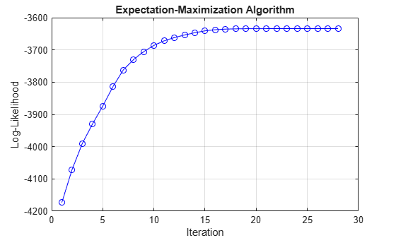
The plot displays the evolution of the loglikelihood with increasing iterations of the EM algorithm. The procedure terminates when one of the stopping criteria is satisfied.
Display an estimation summary of the model.
summarize(EstMdl)
Description
2-Dimensional msVAR Model with 3 Submodels

Switch
Estimated Transition Matrix:
0.501 0.245 0.254
0.204 0.549 0.247
0.188 0.102 0.710

Fit
Effective Sample Size: 999
Number of Estimated Parameters: 14
Number of Constrained Parameters: 0
LogLikelihood: -3634.005
AIC: 7296.010
BIC: 7364.704

Submodels
                           Estimate    StandardError    TStatistic      PValue
                           ________    _____________    __________    ___________

    State 1 Constant(1)    -0.98929       0.023779       -41.603                0
    State 1 Constant(2)     -1.0884       0.030164       -36.083      4.1957e-285
    State 1 AR{1}(1,1)     -0.48446        0.01547       -31.316      2.8121e-215
    State 1 AR{1}(2,1)       0.1835       0.019624        9.3509       8.6868e-21
    State 1 AR{1}(1,2)     0.083953      0.0070162        11.966       5.3839e-33
    State 1 AR{1}(2,2)     -0.72972      0.0089002       -81.989                0
    State 2 Constant(1)     -0.9082       0.030103        -30.17      5.9064e-200
    State 2 Constant(2)      1.9514       0.030483        64.016                0
    State 3 Constant(1)      1.1212       0.044427        25.237      1.5818e-140
    State 3 Constant(2)      1.9561         0.0593        32.986      1.2831e-238
    State 3 AR{1}(1,1)      0.48965       0.023149        21.152       2.6484e-99
    State 3 AR{1}(2,1)      0.22688       0.030899        7.3427       2.0936e-13
    State 3 AR{1}(1,2)     0.095847       0.012005        7.9838       1.4188e-15
    State 3 AR{1}(2,2)      0.72766       0.016024         45.41                0
Display an estimation summary separately for each state.
summarize(EstMdl,1)
Description
2-Dimensional VAR Submodel, State 1

Submodel
                           Estimate    StandardError    TStatistic      PValue
                           ________    _____________    __________    ___________

    State 1 Constant(1)    -0.98929       0.023779       -41.603                0
    State 1 Constant(2)     -1.0884       0.030164       -36.083      4.1957e-285
    State 1 AR{1}(1,1)     -0.48446        0.01547       -31.316      2.8121e-215
    State 1 AR{1}(2,1)       0.1835       0.019624        9.3509       8.6868e-21
    State 1 AR{1}(1,2)     0.083953      0.0070162        11.966       5.3839e-33
    State 1 AR{1}(2,2)     -0.72972      0.0089002       -81.989                0
summarize(EstMdl,2)
Description
2-Dimensional VAR Submodel, State 2

Submodel
                           Estimate    StandardError    TStatistic      PValue
                           ________    _____________    __________    ___________

    State 2 Constant(1)    -0.9082       0.030103         -30.17      5.9064e-200
    State 2 Constant(2)     1.9514       0.030483         64.016                0
summarize(EstMdl,3)
Description
2-Dimensional VAR Submodel, State 3

Submodel
                           Estimate    StandardError    TStatistic      PValue
                           ________    _____________    __________    ___________

    State 3 Constant(1)      1.1212      0.044427         25.237      1.5818e-140
    State 3 Constant(2)      1.9561        0.0593         32.986      1.2831e-238
    State 3 AR{1}(1,1)      0.48965      0.023149         21.152       2.6484e-99
    State 3 AR{1}(2,1)      0.22688      0.030899         7.3427       2.0936e-13
    State 3 AR{1}(1,2)     0.095847      0.012005         7.9838       1.4188e-15
    State 3 AR{1}(2,2)      0.72766      0.016024          45.41                0
Consider the model for the US GDP growth rate in Estimate Markov-Switching Dynamic Regression Model.
Create a Markov-switching dynamic regression model for the naive estimator.
P = NaN(2);
mc = dtmc(P,'StateNames',["Expansion" "Recession"]);
mdl = arima(0,0,0);
Mdl = msVAR(mc,[mdl; mdl]);
Create a fully specified Markov-switching dynamic regression model that has the same structure as Mdl, but set all estimable parameters to initial values.
P0 = 0.5*ones(2);
mc0 = dtmc(P0,'StateNames',Mdl.StateNames);
mdl01 = arima('Constant',1,'Variance',1);
mdl02 = arima('Constant',-1,'Variance',1);
Mdl0 = msVAR(mc0,[mdl01; mdl02]);
Load the US GDP data set. Preprocess the data.
load Data_GDP
qrate = diff(Data(2:230))./Data(2:229); % Quarterly rate
arate = 100*((1 + qrate).^4 - 1);       % Annualized rate
Fit the model Mdl to the annualized rate series arate. Specify Mdl0 as the model containing the initial estimable parameter values.
EstMdl = estimate(Mdl,Mdl0,arate);
Return an estimation summary table.
results = summarize(EstMdl)
results=2×4 table
                           Estimate     StandardError    TStatistic      PValue
                           _________    _____________    __________    ___________

    State 1 Constant(1)       4.9015       0.23023          21.289     1.4301e-100
    State 2 Constant(1)    0.0084884        0.2359        0.035983          0.9713
results is a table containing estimates and inferences for all submodel coefficients.
Identify significant coefficient estimates.
results.Properties.RowNames(results.PValue < 0.05)
ans = 1×1 cell array
    {'State 1 Constant(1)'}
Input Arguments
Output Arguments
Algorithms
estimate implements
a version of Hamilton's Expectation-Maximization (EM) algorithm, as described in [3]. The standard errors, loglikelihood, and
information criteria are conditional on optimal parameter values in the estimated transition
matrix Mdl.Switch. In particular, standard errors do not account for
variation in estimated transition probabilities.
References
[2] Hamilton, J. D. "Analysis of Time Series Subject to Changes in Regime." Journal of Econometrics. Vol. 45, 1990, pp. 39–70.
[3] Hamilton, James D. Time Series Analysis. Princeton, NJ: Princeton University Press, 1994.
[4] Hamilton, J. D. "Macroeconomic Regimes and Regime Shifts." In Handbook of Macroeconomics. (H. Uhlig and J. Taylor, eds.). Amsterdam: Elsevier, 2016.
Version History
Introduced in R2021b