La traduzione di questa pagina non è aggiornata. Fai clic qui per vedere l'ultima versione in inglese.

Stima dei modelli di processo

Stimare dei modelli di processo a tempo continuo per un sistema a singolo-input, singolo-output (SISO) nel dominio del tempo o della frequenza nel Live Editor

Descrizione

L'attività Estimate Process Model (Stima dei modelli di processo) consente di stimare e validare un modello di processo per sistemi SISO in modo interattivo. È possibile definire e variare la struttura del modello e specificare parametri opzionali, come la gestione della condizione iniziale e i metodi di ricerca. L'attività genera automaticamente il codice MATLAB^® per lo script live. Per ulteriori informazioni sulle attività del Live Editor in generale, vedere Add Interactive Tasks to a Live Script.

I modelli di processo sono semplici funzioni di trasferimento a tempo continuo che descrivono la dinamica del sistema lineare. Gli elementi del modello di processo includono il guadagno statico, le costanti di tempo, i ritardi di tempo, l'integratore e il processo zero.

I modelli di processo sono molto diffusi per descrivere la dinamica del sistema in numerosi settori e sono applicabili a vari ambienti di produzione. I vantaggi di questi modelli sono la semplicità, il supporto per la stima del ritardo di trasporto e la facilità di interpretazione dei coefficienti del modello, come poli e zeri. Per ulteriori informazioni sulla stima del modello di processo, vedere What Is a Process Model?

L'attività Estimate Process Model (Stima dei modelli di processo) è indipendente dall'app più generale System Identification. Utilizzare l'app System Identification quando si desidera calcolare e confrontare le stime per più strutture del modello.

Per iniziare, caricare i dati dell'esperimento che contengono i dati di input e output nel workspace di MATLAB, quindi importare i dati nell'attività. Selezionare poi la struttura del modello da stimare. L'attività offre controlli e grafici che consentono di sperimentare diverse strutture di modelli e di confrontare in che misura l'output di ciascun modello si adatta alle misure.

Funzioni correlate

Il codice generato da Estimate Process Model (Stima dei modelli di processo) usa le seguenti funzioni.

• iddata

• idfrd

  frd (Control System Toolbox)

• procest

• procestOptions

• compare

L'attività stima dei modelli di processo idproc.

Apri l'attività

Per aggiungere l'attività Estimate Process Model (Stima dei modelli di processo) in uno script live nell'Editor di MATLAB:

• Nella scheda Live Editor, selezionare Task > Estimate Process Model.

• In un blocco di codice dello script, digitate una parola chiave pertinente, come process o estimate. Selezionare Estimate Process Model dai completamenti dei comandi suggeriti.

Esempi

Stima dei modelli di processo con l'attività di Live Editor

Utilizzare l'attività di Live Editor Estimate Process Model (Stima dei modelli di processo) per stimare un modello di processo e confrontare l'output del modello con i dati di misurazione.

Impostazione dei dati

Caricare i dati di misurazione tt1 nel workspace di MATLAB. tt1 è una tabella orario che contiene una variabile di input u e una variabile di output y.

load sdata1 tt1

Importazione dei dati nell'attività

Nella sezione Select data (Seleziona dati), impostare Data type (Tipo di dati) su Timetable e Estimation data (Dati di stima) su tt1.

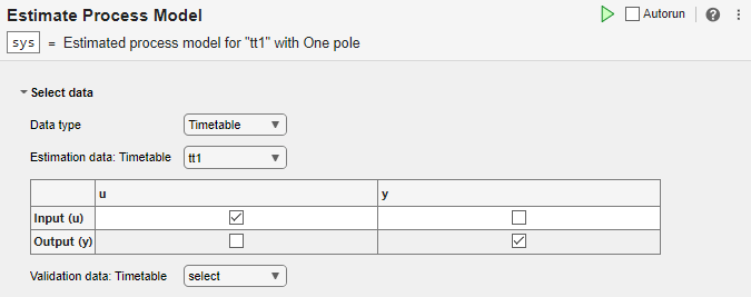
L'attività visualizza una tabella contenente i nomi delle variabili di input e di output tt1.

Stima del modello utilizzando le impostazioni predefinite

Esaminare la struttura del modello e i parametri opzionali.

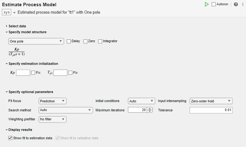
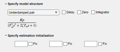
Nella sezione Specify model structure (Specifica struttura del modello), l'opzione predefinita è One Pole, senza ritardi, zero o integratori. Le equazioni sotto i parametri di questa sezione visualizzano la struttura specificata.

Nella sezione Specify estimation initialization (Specifica dell'inizializzazione della stima), i parametri di inizializzazione corrispondenti ai parametri della struttura del modello consentono di impostare i punti di inizio per la stima. Se si seleziona Fix (Fisso), il parametro rimane fisso sul valore specificato. Per questo esempio, non specificare l'inizializzazione. L'attività utilizza quindi i valori predefiniti per i punti di inizio.

Nella sezione Specify optional parameters (Specifica dei parametri opzionali), vengono impostate le opzioni predefinite per la stima del processo.

Eseguire l'attività dalla scheda Live Editor facendo clic sulla freccia verde. È anche possibile selezionare Autorun (Esecuzione automatica) per eseguire automaticamente l'attività ogni volta che si aggiorna un parametro.

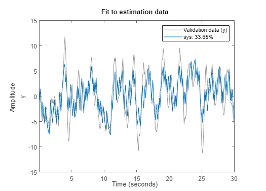
Un grafico mostra i dati di stima, l'output del modello stimato e la percentuale di adattamento.

Sperimentazione delle impostazioni dei parametri

Sperimentare le impostazioni dei parametri e verificare come influenzano l'adattamento.

Ad esempio, aggiungere un ritardo alla struttura One Pole ed eseguire l'attività.

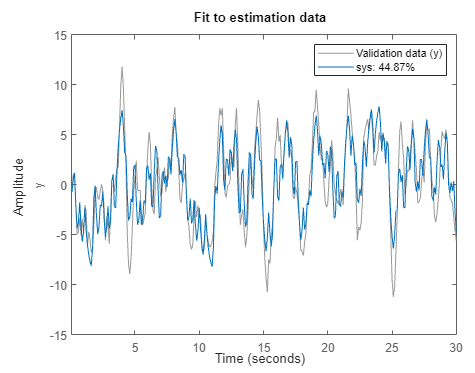
L'adattamento della stima migliora, anche se la percentuale di adattamento è ancora inferiore al 50%.

Provare una diversa struttura del modello. In Specify model structure (Specifica struttura del modello), selezionare Underdamped Pair senza ritardi ed eseguire l'attività.

I risultati dell'adattamento migliorano in modo significativo.

Generazione di codice

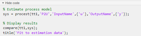
Per visualizzare il codice generato dall'attività, fare clic su in fondo alla sezione dei parametri. Il codice visualizzato riflette la configurazione corrente dei parametri dell'attività.

Utilizzo dell'insieme dei dati di validazione per validare il modello stimato

Utilizzare dati di stima e di validazione separati in modo da poter validare il modello di processo stimato.

Impostazione dei dati

Caricare i dati di misurazione sdata1 nel workspace di MATLAB ed esaminarne il contenuto.

load sdata1 umat1 ymat1 Ts

Dividere i dati in due insiemi, una metà per la stima e una metà per la validazione. L'insieme originale dei dati ha 300 campioni, quindi ogni nuovo insieme di dati ha 150 campioni.

u_est = umat1(1:150);
u_val = umat1(151:300);
y_est = ymat1(1:150);
y_val = ymat1(151:300);
Ts

Ts = 
0.1000

Importazione dei dati nell'attività

Nella sezione Select data (Seleziona dati), impostare Data type (Tipo di dati) su numerico. Impostare il tempo di campionamento su 0.1 secondi. Selezionare gli insiemi di dati appropriati per la stima e la validazione.

Stima e validazione del modello

L'esempio Stima dei modelli di processo con l'attività di Live Editor ottiene i migliori risultati utilizzando la struttura del modello Underdamped Pair. Scegliere la stessa opzione per questo esempio.

Eseguire l'attività. L'esecuzione dell'attività crea due grafici. Il primo grafico mostra i risultati della stima e il secondo quelli della validazione.

L'adattamento ai dati di stima è leggermente peggiore rispetto a Stima dei modelli di processo con l'attività di Live Editor. Nell'esempio attuale, la stima dispone solo della metà dei dati con cui stimare il modello. L'adattamento ai dati di validazione, che rappresenta in modo più generale la validità del modello, è migliore rispetto all'adattamento ai dati di stima.

Parametri

Selezione dei dati

Data Type — Tipo di dati per i dati di input e output

Numeric (predefinito) | Timetable | Frequency | Data Object

L'attività accetta valori di misura numerici campionati in modo uniforme nel tempo. I segnali di input e di output possono contenere più canali. I dati possono essere strutturati come array numerici (per Numeric o Frequency), come tabella orario o oggetto dati, come un oggetto iddata o idfrd. Per i dati di più esperimenti, i dati numerici e quelli relativi alle tabelle orario possono essere strutturati come array di celle. Per gli array di celle di tabelle orario, tutte le tabelle orario devono contenere gli stessi nomi di variabili. Gli oggetti dati gestiscono i dati di più esperimenti internamente.

Il tipo di dati scelto determina la necessità o meno di specificare parametri aggiuntivi.

• Numeric: specificare Sample Time e Start Time nelle unità di tempo selezionate.

• Timetable: non specificare ulteriori parametri in quanto la tabella orario contiene già le informazioni sul tempo di campionamento e di inizio.

• Frequency: specificare Frequency selezionando il nome della variabile di un vettore di frequenza nel workspace di MATLAB. Specificare le unità per questo vettore di frequenza. Specificare Sample Time in secondi.

• Data Object: non specificare ulteriori parametri in quanto l'oggetto dati contiene già le informazioni sul campionamento del tempo o della frequenza.

Estimation and Validation data: Input (u) and Output (y) — Nomi delle variabili di input e output dei dati per la stima o la validazione

nomi validi delle variabili

Selezionare i nomi delle variabili di input e output dalle scelte del workspace di MATLAB. Utilizzare questi parametri quando Data Type è Numeric o Frequency.

Specificare i dati di validazione è opzionale ma consigliato.

Estimation and Validation data: Timetable — Nome della variabile della tabella orario da utilizzare per la stima o la validazione

nome valido della variabile

Selezionare il nome della variabile della tabella orario dalle scelte del workspace di MATLAB. Utilizzare questo parametro quando Data Type è Timetable. L'attività visualizza i nomi delle variabili della tabella orario per l'input e l'output. Le tabelle orario di stima e validazione devono contenere gli stessi nomi di variabili.

Estimation and Validation Data Object — Nome della variabile dell'oggetto dati (oggetto iddata, idfrd o frd) contenente input e output dei dati da utilizzare per la stima o la validazione

nome valido della variabile

Selezionare il nome della variabile dell'oggetto dati dalle scelte del workspace di MATLAB. Utilizzare questo parametro quando Data Type è Data Object.

Specifica struttura del modello

Structure — Zero e poli nel modello

One Pole (predefinito) | Two Real Poles | Underdamped Pair | Underdamped Pair + Real Pole

L'attività consente di specificare una delle quattro strutture di base. Queste strutture vanno da un semplice processo di primo ordine a un processo più dinamico di secondo o terzo ordine con poli complessi coniugati (sottosmorzati).

• One Pole

• Two Real Poles

• Underdamped Pair

• Underdamped Pair + Real Pole

Delay — Includere il ritardo di trasporto

off (predefinito) | on

Includere il ritardo di trasporto, o il ritardo di input-output, di un campione. Il ritardo di trasporto è anche conosciuto come tempo morto.

Zero — Includere un processo zero

off (predefinito) | on

Includere un processo zero nel numeratore.

Integrator — Includere un integratore

off (predefinito) | on

Includere un integratore, rappresentato da un termine aggiuntivo 1/ s. Includere un integratore crea un processo autoregolante.

Specifica dell'inizializzazione della stima

Initial Values — Valori iniziali dei parametri della struttura

0 | valori dei parametri

Specificare i valori iniziali della stima e se tali valori devono essere fissi o stimati. I valori da specificare dipendono dalla struttura del modello e dalle specifiche per Delay e Zero. Sotto Specify model structure, l'attività mostra l'equazione che rappresenta il sistema specificato. Questa equazione contiene tutti i parametri che possono essere stimati e che è possibile inizializzare o correggere. I possibili parametri sono i seguenti:

• Kp: guadagno statico

• T_p1: costante di tempo per il primo polo reale

• T_p2: costante di tempo per il secondo polo reale

• Tω: costante di tempo per poli complessi, uguale all'inverso della frequenza naturale

• ζ: coefficiente di smorzamento per poli complessi

• T_d: Ritardo di trasporto

• T_z: costante di tempo per il processo zero

Tutti i parametri basati sul tempo sono espressi nelle unità di tempo selezionate per Sample Time.

Specifica dei parametri opzionali

Fit Focus — Minimizzare l'errore di previsione o l'errore di simulazione

Prediction (predefinito) | Simulation

Fit focus specifica quale errore deve essere minimizzato nella funzione di perdita durante la stima.

• Prediction: minimizzare l'errore di previsione di uno step in avanti tra gli output misurati e quelli previsti. Questo approccio di stima si focalizza sulla creazione di un buon modello predittivo per gli input e gli output della stima. Il focus sulla previsione produce generalmente i migliori risultati di stima poiché utilizza sia le misurazioni di input che quelle di output, tenendo quindi in considerazione i disturbi.

• Simulation: minimizzare l'errore tra output misurati e di simulazione. Questo approccio di stima si focalizza sulla creazione di un modello di risposta simulato che si adatti bene agli input e agli output della stima. Il focus sulla simulazione è generalmente più adatto per la validazione, specialmente con insiemi di dati non utilizzati per la stima originale.

Initial Conditions — Gestire le condizioni iniziali

Auto (predefinito) | Zero | Estimate | Backcast

Impostare questa opzione quando si desidera scegliere un metodo specifico per l'inizializzazione del modello. Con l'impostazione predefinita di Auto, il software sceglie il metodo in base ai dati di stima. Le scelte sono le seguenti:

• Zero: lo stato iniziale è impostato su zero.

• Estimate: lo stato iniziale viene trattato come un parametro di stima indipendente.

• Backcast: lo stato iniziale viene stimato utilizzando la migliore approssimazione ai minimi quadrati.

Input Intersampling — Comportamento intercampione per il segnale di input

Zero-order hold (predefinito) | Triangle approximation | Band-limited

L'intercampionamento dell'input è una proprietà dei dati di input. L'attività utilizza questa proprietà nella stima dei modelli di processo. Specificare Input Intersampling quando il tipo di dati è Time o Frequency. Se si sta utilizzando un oggetto iddata, l'oggetto contiene già le informazioni di intercampionamento. Le scelte per questa proprietà sono le seguenti:

• Zero-order hold: segnale di input costante a tratti tra i campioni

• Triangle approximation: segnale di input lineare a tratti tra i campioni, conosciuto anche come blocco di primo ordine

• Band-limited: il segnale di input ha potenza zero al di sopra della frequenza di Nyquist

Search Method — Modalità di ricerca numerica per la stima iterativa dei parametri

Auto (predefinito) | Gauss-Newton | Adaptive Gauss-Newton | Levenberg-Marquardt | Gradient search | Trust-Region Reflective Newton | Pattern Search | Sequential Quadratic Programming (SQP) | Interior-Point

I metodi di ricerca numerica disponibili per la stima iterativa dei parametri sono i seguenti:

Metodo di ricerca	Descrizione
Auto	Per ogni iterazione, il software passa in rassegna i metodi fino a trovare la prima direzione di discesa che porta a una riduzione del costo di stima.
Gauss-Newton	I valori singolari della matrice jacobiana inferiori a GnPinvConstant*eps*max(size(J))*norm(J) vengono scartati durante il calcolo della direzione di ricerca. J è la matrice jacobiana. La matrice hessiana è approssimata come JTJ. Se questa direzione non mostra alcun miglioramento, la funzione prova la direzione del gradiente.
Adaptive Gauss-Newton	Gli autovalori inferiori a gamma*max(sv) della hessiana vengono ignorati, dove sv contiene i valori singolari della hessiana. La direzione di Gauss-Newton viene calcolata nel sottospazio rimanente. gamma ha il valore iniziale InitialGnaTolerance (per ulteriori informazioni, vedere Advanced in 'SearchOptions'). Questo valore viene aumentato del fattore LMStep ogni volta che la ricerca non riesce a trovare un valore inferiore del criterio in meno di cinque bisezioni. Questo valore viene diminuito del fattore 2*LMStep ogni volta che una ricerca ha esito positivo senza alcuna bisezione.
Levenberg-Marquardt	Ogni valore del parametro è -pinv(H+d*I)*grad dal valore precedente. H è la hessiana, I è la matrice di identità e grad è il gradiente. d è un numero che viene aumentato fino a quando non viene trovato un valore inferiore del criterio. Per questo metodo è necessario disporre del software Optimization Toolbox™. Per ulteriori informazioni, vedere Levenberg-Marquardt Method (Optimization Toolbox).
Gradient search	Ricerca dei minimi quadrati con la discesa più ripida.
Trust-Region Reflective Newton	Un risolutore non lineare vincolato. Per questo risolutore è necessario disporre del software Optimization Toolbox. Per ulteriori informazioni, vedere fmincon Trust Region Reflective Algorithm (Optimization Toolbox).
Pattern Search	Risolutore per la non linearità senza gradienti ben definiti. Per questo risolutore è necessario disporre del software Global Optimization Toolbox. Per ulteriori informazioni, vedere patternsearch (Global Optimization Toolbox).
Sequential Quadratic Programming (SQP)	Un risolutore non lineare vincolato. Per questo risolutore è necessario disporre del software Optimization Toolbox. Per ulteriori informazioni, vedere fmincon SQP Algorithm (Optimization Toolbox).
Interior-Point	Un risolutore non lineare vincolato. Per questo risolutore è necessario disporre del software Optimization Toolbox. Per ulteriori informazioni, vedere fmincon Interior Point Algorithm (Optimization Toolbox).

Max. Iterations — Numero massimo di iterazioni durante la minimizzazione dell'errore

20 (predefinito) | intero positivo

Impostare il numero massimo di iterazioni durante la minimizzazione dell'errore. Le iterazioni si interrompono quando si raggiunge Max. Iterations o quando viene soddisfatto un altro criterio di arresto, come Tolerance.

Tolerance — Percentuale minima di miglioramento atteso dell'errore

0.01 (predefinito) | intero positivo

Quando la percentuale di miglioramento atteso è inferiore a Tolerance, le iterazioni si interrompono.

Weighting Prefilter — Pre-filtro di ponderazione per la funzione di perdita

No filter (predefinito) | Passband(s) | LTI Filter | Frequency weights vector

Impostare questa opzione quando si desidera applicare un pre-filtro di ponderazione alla funzione di perdita che l'attività minimizza quando si stima il modello. Quando si seleziona un'opzione, è inoltre necessario selezionare la variabile associata nel workspace che contiene le informazioni del filtro. Le opzioni disponibili dipendono dal dominio dei dati.

Pre-filtro di ponderazione	Dominio dei dati	Informazioni sul filtro
No Filter	Tempo e frequenza
Passbands	Tempo e frequenza	Intervalli di banda passante, specificati come vettore riga 1x2 o come matrice nx2, dove n è il numero di bande passanti
LTI Filter	Tempo e frequenza	Modello LTI SISO
Frequency Weights Vector	Frequenza	Pesi della frequenza, specificati come vettore colonna della stessa lunghezza del vettore di frequenza

Ad esempio, si supponga di eseguire una stima con dati SISO nel dominio della frequenza e che nel workspace di MATLAB sia presente un vettore colonna W contenente i pesi di frequenza per il pre-filtro. Nell'attività, selezionare Weighting prefilter > Frequency weights vector e la variabile W.

Visualizzazione dei risultati

Output Plot — Confronto grafico tra modello e output misurati

on (predefinito) | off

Tracciare un confronto tra l'output del modello e i dati misurati originali, insieme alla percentuale di adattamento. Se sono presenti dati di validazione separati, un secondo grafico confronta la risposta del modello rispetto all'input dei dati di validazione con l'output misurato dall'insieme dei dati di validazione.

Cronologia versioni

Introdotto in R2019b

R2025a: Nuovo risolutore di pattern di ricerca disponibile per la stima

Ora è possibile stimare un sistema che presenta una non linearità senza un gradiente ben definito impostando Search Method su Pattern Search. Per questo metodo è necessario disporre del software Global Optimization Toolbox.

R2024b: Supporto dati per più esperimenti

L'attività di Live Editor Estimate Process Model (Stima dei modelli d processo) ora supporta i dati per più esperimenti.

R2023b: Accettazione dei dati di stima basati sulla tabella orario

L'attività viene aggiornata per accettare dati nel dominio del tempo sotto forma di tabella orario. L'attività continua ad accettare anche dati numerici nel dominio del tempo, con l'opzione del tipo di dati Numeric.

Vedi anche

timetable | iddata | procest | procestOptions | compare | idproc | idfrd | frd (Control System Toolbox)