detrend
Subtract offset or trend from time-domain signals contained in
iddata objects
Syntax
Description
detrend subtracts offsets or linear trends from
time-domain input-output data represented in iddata objects.
detrend either computes the trend data to subtract, or
subtracts the trend that you specify.
For a more general detrending function that does not require
iddata objects, see detrend.
data_d = detrend(data,1,brkpt)brkpt.
The second argument, which corresponds to Type, must be
1.
With this syntax, you cannot retrieve the resulting piecewise-linear trend information as an output.
Examples
Remove biases from steady-state signals in an iddata object by using detrend to compute and subtract the mean values of the input and output.
Load the input and output time series data y2 and u2. Construct the iddata object data2, using the data and a sample time of 0.08 seconds.
load dryer2 y2 u2
data2 = iddata(y2,u2,0.08);
Use detrend to both compute the mean values and subtract them from input and output signals. Use the input argument Tr to store the computed trend information. Plot the original data and detrended data together.
[data2_d,Tr] = detrend(data2);
plot(data2,data2_d)
legend('Original Data','Detrended Data')

The detrended data has shifted by about 5 units. Inspect Tr to obtain the precise mean values that detrend computed and subtracted. These values are returned in the InputOffset and OutputOffset properties.
Tr
Trend specifications for data "data2" with 1 input(s), 1 output(s), 1 experiment(s):
        DataName: 'data2'
     InputOffset: 5.0000
    OutputOffset: 4.8901
      InputSlope: 0
     OutputSlope: 0
The mean of the original input is higher than the mean of the original output.
Remove the linear trend from a signal in an iddata object, and overlay the trendline on a before-and-after data plot.
Load and plot signal data from the file lintrend2. For this example, only output data is provided in iddata object dataL.
load lintrend2 dataL
plot(dataL,'b')

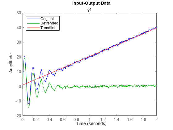
The plot shows a clear linear trend in the data. Use detrend linear option (Type = 1) to subtract the trend from the data. detrend fits the data and determines the linear trend to subtract. Include the TrendInfo object Tr as an output argument so you can see what detrend subtracts.
[dataL_d,Tr] = detrend(dataL,1);
Plot the detrended data against the original data.
hold on
plot(dataL_d,'g')
legend('Original','Detrended','Location','northwest')

The linear trend has been removed. Inspect Tr to get more information about the removed trend.
Tr
Trend specifications for data "dataL" with 0 input(s), 1 output(s), 1 experiment(s):
        DataName: 'dataL'
     InputOffset: [1×0 double]
    OutputOffset: 0.8888
      InputSlope: [1×0 double]
     OutputSlope: 19.3830
The OutputOffset and the OutputSlope properties provide the parameters of the line that detrend removed. You can reconstruct this line, and then overlay it on the before-and-after data plot. The SamplingInstants property of DataL provides the timepoints associated with the data.
m = Tr.OutputSlope
m =
19.3830
b = Tr.OutputOffset
b =
0.8888
t = dataL.SamplingInstants;
TrLn = m*t+b;
plot(t,TrLn,'r')
legend('Original','Detrended','Trendline','Location','northwest')

Remove known offsets from an input-output signal pair contained in an iddata object.
Detrend can compute and subtract the mean values for input and output signals, resulting in zero-mean detrended signals. However, if you already know you have specific data offsets beforehand, you can have detrend subtract these from your signals instead. Specifying the offsets also allows you to retain a non-zero operating point in the detrend result.
Load SISO data containing vectors u2 and y2. For this example, suppose that you know both signals have an offset of 4 from the expected operating point of 1. Combine these vectors into an iddata object, using a sample time of 0.08 seconds, and plot it.
load dryer2 u2 y2
data = iddata(y2,u2,0.08);
plot(data)

The known offset of 4 (from operating point 1) is visible in the plots. You can construct a TrendInfo object to capture this offset, using the function getTrend.
Create the TrendInfo object, and then set its offset properties.
T = getTrend(data);
T.InputOffset = 4;
T.OutputOffset = 4
Trend specifications for data "data" with 1 input(s), 1 output(s), 1 experiment(s):
        DataName: 'data'
     InputOffset: 4
    OutputOffset: 4
      InputSlope: 0
     OutputSlope: 0
Use detrend to subtract the offset from the data. Plot it alongside the original data.
data_d = detrend(data,T);
hold on
plot(data_d)
legend("Interpreter","none")

The offset of 4 has been removed.
Detrend data with segmented piecewise-linear trends by specifying breakpoints to delimit the segments.
Most of the detrend syntaxes assume and compute a single trend for each of the signals. However, in some cases there are discontinuities in the linear trends, caused by test configuration changes, environmental conditions, or other influences. When the signal displays such segmentation, you can have detrend operate on the test segments independently. To do so, specify breakpoints in the brkpt input argument. These are the indices to the timepoints in the signal at which linear trends change slope.
You may know these breakpoints up front, based on changes that you know occurred during data collection. Alternatively, you may need to approximate them by inspecting the data itself.
Load the data, inspect its structure and contents, and plot it. This data consists of output data only in the iddata object dataLb2.
load brkTrend dataLb2
dataLb2
dataLb2 =
Time domain data set with 512 samples.
Sample time: 0.00390625 seconds

Outputs      Unit (if specified)
   y1

Data Properties
plot(dataLb2)

For this example, the data has known breakpoints at indices [100 300]. Applying the sample time (property Ts), these breakpoints correspond to the actual timepoints as follows:
brkpt=[100 300];
brkpt_time = brkpt*dataLb2.Ts
brkpt_time = 1×2

    0.3906    1.1719
Detrend the data using brkpt.
dataLb2_d = detrend(dataLb2,1,brkpt);
Plot the original and detrended data.
plot(dataLb2,dataLb2_d)
legend('Original Data','Detrended Data')

The linear trend segments have been removed.
Apply a unique set of breakpoints to each experiment when you detrend a Multiexperiment dataset.
Experiments within a multiexperiment dataset may contain unique linear trending discontinuities. You can apply a unique set of breakpoints to each experiment by expressing them in a cell array.
Load the data, which consists of:
datmult, a multiexperimentiddataobject containing three experiments (output only)bpn vectors, which provide known breakpoints for each experiment in the form of indices to timepoints
load multiexpdt datmult bp1 bp2 bp3
datmult
datmult =
Time domain data set containing 3 experiments.

Experiment   Samples      Sample Time
   exp1         250            1
   exp2         320            1
   exp3         350            1

Outputs      Unit (if specified)
   y1

Data Properties
bp1,bp2,bp3
bp1 = 1×2

    50   200
bp2 =
100
bp3 =

     []
Plot the data. There are significant differences among the streams, and they drift at different rates from zero mean.
plot(datmult)
legend

For this set of experiments, it is known that there is unique trending for each run and unique discontinuities indicated by the bp vectors.
detrend can incorporate these unique characteristics if the bp information is provided as a cell array.
Construct the cell array.
bpcell = {bp1;bp2;bp3}bpcell=3×1 cell array
{[ 50 200]}
{[ 100]}
{0×0 double}
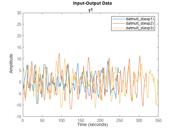
Apply detrend and plot the result, using the same scale as the original plot.
datmult_d = detrend(datmult,1,bpcell);
figure
plot(datmult_d)
axis([0,inf,-15,30])
legend

The experimental data are now better aligned, and do not drift significantly away from zero mean.
Apply different trend types to the input and output signals contained in an iddata object.
Detrend assumes that the same type of trend applies to both input and output signals. In some cases, there may be a trend type that is present in only one signal. You can perform detrend individually on each signal by extracting the signals into separate iddata objects. Apply detrend to each object using its individual signal trend type. Then reassemble the results back into a single detrended iddata object.
Load, examine, and plot the data in iodatab.
load septrend iodatab;
iodatab
iodatab =
Time domain data set with 1000 samples.
Sample time: 0.08 seconds

Outputs      Unit (if specified)
   y1

Inputs       Unit (if specified)
   u1

Data Properties
plot(iodatab)
hold on
Both input and output plots show a bias. However, the output plot also shows an inverted V-shape trend that is not present in the input data.
Separate the input data and the output data into separate objects for detrending, using the iddata general data-selection form (see Representing Time- and Frequency-Domain Data Using iddata Objects):
data(samples,outputchannels,inputchannels)
idatab = iodatab(:,[],:);
odatab = iodatab(:,:,[]);
Remove the bias from the input data, using detrend to calculate and subtract the mean.
idatab_d = detrend(idatab,0);
Remove the bias and the inverted-V trend from the output data, using the midpoint index 500 as a breakpoint.
odatab_d = detrend(odatab,1,500);
Combine the detrended input and output data into a single iddata object.
iodatab_d = [odatab_d,idatab_d];
Overlay the detrended data on the original data.
plot(iodatab_d)
legend("Interpreter","none")

The input and output data now contain neither bias nor V-shape trend.
Input Arguments
Time-domain input-output data, specified as an iddata
object containing one or more sets of time-domain signals. The
iddata object can contain SISO, MIMO, or
multiexperiment data. The signal sets can contain either input and output
data, or output data only.
Trend type to be subtracted, specified as one of:
0 — Compute and subtract the mean value
1 — Compute and subtract the linear trend (least-squares fit)
TrendInfoobject — subtract the trend you specify in theTrendInfoobject. UsegetTrendto create aTrendInfoobject. For an example, see Remove Specified Offsets from Signals.
Timepoint locations of trending discontinuities (breakpoints), specified as:
An integer row vector — For single-experiment SISO and MIMO datasets. Doing so applies a single set of breakpoints to all input and output signals. For an example, see Remove Segmented Linear Trends from Signals by Using Breakpoints.
A cell array containing individually-sized integer row vectors — For multiple-experiment datasets. Doing so applies a unique set of breakpoints to the output and input signals for each experiment. For an example, see Detrend Multiexperiment Signals Using Multiple-Breakpoint Sets.
Output Arguments
Detrended signals, returned as an iddata object.
Dimensions of the contents are the same as dimensions of the contents of
data.
Version History
Introduced before R2006a
MATLAB Command
You clicked a link that corresponds to this MATLAB command:
Run the command by entering it in the MATLAB Command Window. Web browsers do not support MATLAB commands.
Seleziona un sito web
Seleziona un sito web per visualizzare contenuto tradotto dove disponibile e vedere eventi e offerte locali. In base alla tua area geografica, ti consigliamo di selezionare: .
Puoi anche selezionare un sito web dal seguente elenco:
Come ottenere le migliori prestazioni del sito
Per ottenere le migliori prestazioni del sito, seleziona il sito cinese (in cinese o in inglese). I siti MathWorks per gli altri paesi non sono ottimizzati per essere visitati dalla tua area geografica.
Americhe
- América Latina (Español)
- Canada (English)
- United States (English)
Europa
- Belgium (English)
- Denmark (English)
- Deutschland (Deutsch)
- España (Español)
- Finland (English)
- France (Français)
- Ireland (English)
- Italia (Italiano)
- Luxembourg (English)
- Netherlands (English)
- Norway (English)
- Österreich (Deutsch)
- Portugal (English)
- Sweden (English)
- Switzerland
- United Kingdom (English)