Convert Coastline Data (GSHHG) to Shapefile Format
The Global Self-Consistent Hierarchical High-Resolution Geography (GSHHG) data set [1] is a collection of geographic data that includes the boundaries of coastlines, lakes, and major rivers. GSHHG data is useful for creating base layers for maps and for performing analyses that require operations such as geographic searches and geometric quantities.
This example shows how to:
Extract a subset of data from the GSHHG data set.
Represent the data using polygon shapes.
Merge the polygons that represent land areas and lakes.
Save the merged data to a shapefile.
Index Coarse-Resolution GSHHG Data
Extract a file containing coarse GSHHG data from a GNU zipped file. Read the file into the workspace as a geographic data structure array.
files = gunzip("gshhs_c.b.gz");
filename = files{1};
Create an index file that accelerates future calls to the gshhs function. Note that, when you create an index file by using the "createindex" option, the gshhs function does not extract data.
indexfile = gshhs(filename,"createindex");Read GSHHG Data
Specify the latitude and longitude limits of a region surrounding South America. Then, read GSHHG data for the region into the workspace as a geographic data structure array.
latlim = [-60  15];
lonlim = [-90 -30];
S = gshhs(filename,latlim,lonlim);
Convert the structure array into a geospatial table by using the struct2geotable function. A geospatial table is a table or timetable object that contains a Shape variable and attribute variables.
GT = struct2geotable(S);
Examine GSHHG Data
Note that the Shape variable contains a polygon shape in geographic coordinates.
GT.Shape
ans=155×1 geopolyshape array with properties:
              NumRegions: [155×1 double]
                NumHoles: [155×1 double]
                Geometry: "polygon"
    CoordinateSystemType: "geographic"
           GeographicCRS: []
      ⋮
GSHHS data includes multiple shoreline levels:
Level 1 polygons represent land areas.
Level 2 polygons represent lakes.
Level 3 polygons represent islands within lakes.
Level 4 polygons represent ponds within islands that are within lakes.
Find the shoreline levels in the South America GSHHG data by querying the Level variable of the geospatial table. The result indicates that the South America GSHHS data includes level 1, 2, and 3 polygons.
levels = GT.Level;
unique(levels)
ans = 3×1

     1
     2
     3
Alternatively, you can find the interpretation of the shoreline levels in the South America GSHHG data by querying the LevelString variable of the geospatial table. The result also indicates that the South America GSHHS data includes islands in lakes (level 3), lakes (level 2), and land (level 1).
levelstrings = GT.LevelString;
unique(levelstrings)
ans = 3×1 cell
    {'island_in_lake'}
    {'lake'          }
    {'land'          }
Display Land Areas and Lakes
Create two subtables from the geospatial table. Create the first subtable from the table rows that represent land areas. Create the second subtable from the table rows that represent lakes.
idxL1 = (levels == 1);
L1 = GT(idxL1,:);

idxL2 = (levels == 2);
L2 = GT(idxL2,:);
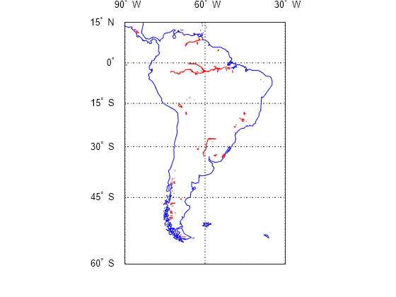
Display the land areas and the lakes on a map. Display the land areas using polygons with blue outlines, and display the lakes using polygons with red outlines. Note that the lake polygons include other extended bodies of water.
figure
worldmap(latlim,lonlim)
mlabel off
geoshow(L1,EdgeColor="#0072BD",FaceColor="none")
geoshow(L2,EdgeColor="#A2142F",FaceColor="none")

Merge Land Areas and Lakes
Merge the land area polygons and the lake polygons, such that the result is a collection of land area polygons with holes that represent lakes.
For each row of the land area and lake geospatial tables:
Get the bounding boxes for the land area and lake polygons.
Determine if the bounding boxes overlap by using the
boxesIntersecthelper function. This step improves the performance of the code by omitting calculations on nonoverlapping polygon shapes.If the bounding boxes overlap, create holes in the land area polygon by finding the difference of the land area polygon and the lake polygon.
In the land area geospatial table, replace the original land area polygon with the updated land area polygon.
for landIDX = 1:height(L1)
    % land area bounding box
    landBBOX = L1.BoundingBox{landIDX};
    for lakeIDX = 1:height(L2)
        % lake bounding box
        lakeBBOX = L2.BoundingBox{lakeIDX};
        % determine if bounding boxes overlap
        if boxesIntersect(landBBOX,lakeBBOX)
            landShape = L1.Shape(landIDX);
            lakeShape = L2.Shape(lakeIDX);
            % calculate difference of land area and lake polygons
            mergedShape = subtract(landShape,lakeShape);
            % replace original land area polygon
            L1.Shape(landIDX) = mergedShape;
        end
    end
end
Write Merged Data to Shapefile
Write the updated geospatial table to a shapefile. Note that the shapefile consists of multiple files: a main file (.shp), an index file (.shx), and an attribute file (.dbf).
filename = "gshhs_c_SouthAmerica.shp";
shapewrite(L1,filename)
Validate Shapefile
Validate the shapefile by reading and displaying the data stored in the file.
Read the shapefile into a new geospatial table.
GT2 = readgeotable("gshhs_c_SouthAmerica.shp",CoordinateSystemType="geographic");
Display the variables names of the new table. Note that, due to character limits in the attribute file (.dbf) specification, the original attribute names FormatVersion and CrossesGreenwich are truncated to 11 characters.
GT2.Properties.VariableNames'
ans = 13×1 cell
    {'Shape'      }
    {'South'      }
    {'North'      }
    {'West'       }
    {'East'       }
    {'Area'       }
    {'Level'      }
    {'LevelString'}
    {'NumPoints'  }
    {'FormatVersi'}
    {'Source'     }
    {'CrossesGree'}
    {'GSHHS_ID'   }
Display the merged data on a map. Note that the land area polygons contain holes that represent lakes and other extended bodies of water.
figure
worldmap(latlim,lonlim)
ax = gca;
setm(ax,"FFaceColor","#4DBEEE")
mlabel off
geoshow(GT2,FaceColor="#77AC30")

References
[1] "GSHHG - A Global Self-Consistent, Hierarchical, High-Resolution Geography Database." Accessed October 22, 2024. https://www.soest.hawaii.edu/pwessel/gshhg/.
Helper Function
The boxesIntersect helper function returns a logical 1 if the bounding boxes specified by bbox1 and bbox2 intersect, and 0 otherwise. bbox1 and bbox2 are 2-by-2 matrices of the form [lonmin latmin; lonmax latmax].
function tf = boxesIntersect(bbox1,bbox2)
    tf = ~(any(bbox1(2,:) < bbox2(1,:)) || any(bbox2(2,:) < bbox1(1,:)));
end