Import NetCDF Files and OPeNDAP Data
You can read data from a netCDF file in several ways. Programmatically, you can use the MATLAB® high-level netCDF functions or the netCDF library namespace of low-level functions. Interactively, you can use the Import Data Live Editor task or (in MATLAB Online™) the Import Tool app.
MATLAB NetCDF Capabilities
Network Common Data Form (NetCDF) is a set of software libraries and machine-independent data formats that support the creation, access, and sharing of array-oriented scientific data. NetCDF is used by a wide range of engineering and scientific fields that want a standard way to store data so that it can be shared.
MATLAB high-level functions simplify the process of importing data from a NetCDF file or an OPeNDAP NetCDF data source. MATLAB low-level functions enable more control over the importing process, by providing access to the routines in the NetCDF C library. To use the low-level functions effectively, you should be familiar with the NetCDF C Interface. The NetCDF documentation is available at the Unidata website.
Note
For information about importing Common Data Format (CDF) files, which have a separate, incompatible format, see Import CDF Files Using Low-Level Functions.
Security Considerations When Connecting to an OPeNDAP Server
It is highly recommended that you connect only to trusted OPeNDAP servers. Since R2020b, the MATLAB NetCDF interface connects only to trusted data access protocol (DAP) endpoints by default by performing server certificate and host name validations. Previously, when you accessed an OPeNDAP server, both the server certificate and host name validation were disabled by default.
If you would like to disable the server certificate and host name validation, add
the following line in a .dodsrc file in the current
directory:
[mylocaltestserver.lab] HTTP.SSL.VALIDATE=0
This makes the MATLAB NetCDF interface connect to the OPeNDAP server whose name is specified
in the URI mylocaltestserver.lab without performing any
validations on the server certificate or host name. This change persists in future
MATLAB sessions.
Read from NetCDF File Using High-Level Functions
This example shows how to display and read the contents of a NetCDF file, using high-level functions.
Display the contents of the sample NetCDF file,
example.nc.
ncdisp('example.nc')Source:
\\matlabroot\toolbox\matlab\demos\example.nc
Format:
netcdf4
Global Attributes:
creation_date = '29-Mar-2010'
Dimensions:
x = 50
y = 50
z = 5
Variables:
avagadros_number
Size: 1x1
Dimensions:
Datatype: double
Attributes:
description = 'this variable has no dimensions'
temperature
Size: 50x1
Dimensions: x
Datatype: int16
Attributes:
scale_factor = 1.8
add_offset = 32
units = 'degrees_fahrenheit'
peaks
Size: 50x50
Dimensions: x,y
Datatype: int16
Attributes:
description = 'z = peaks(50);'
Groups:
/grid1/
Attributes:
description = 'This is a group attribute.'
Dimensions:
x = 360
y = 180
time = 0 (UNLIMITED)
Variables:
temp
Size: []
Dimensions: x,y,time
Datatype: int16
/grid2/
Attributes:
description = 'This is another group attribute.'
Dimensions:
x = 360
y = 180
time = 0 (UNLIMITED)
Variables:
temp
Size: []
Dimensions: x,y,time
Datatype: int16ncdisp displays all the groups, dimensions, and
variable definitions in the file. Unlimited dimensions are identified with
the label, UNLIMITED.
Read data from the peaks variable.
peaksData = ncread('example.nc','peaks');
Display information about the peaksData output.
whos peaksDataName Size Bytes Class Attributes peaksData 50x50 5000 int16
Read the description attribute associated with the
variable.
peaksDesc = ncreadatt('example.nc','peaks','description')
peaksDesc =

z = peaks(50);
Create a three-dimensional surface plot of the variable data. Use the
value of the description attribute as the title of the
figure.
surf(double(peaksData))
title(peaksDesc);
Read the description attribute associated with the
/grid1/ group. Specify the group name as the second
input to the ncreadatt function.
g = ncreadatt('example.nc','/grid1/','description')
g =

This is a group attribute.
Read the global attribute, creation_date. For global
attributes, specify the second input argument to
ncreadatt as '/'.
creation_date = ncreadatt('example.nc','/','creation_date')
creation_date =

29-Mar-2010
Find All Unlimited Dimensions in NetCDF File
This example shows how to find all unlimited dimensions in a group in a NetCDF file, using high-level functions.
Get information about the /grid2/ group in the sample
file, example.nc, using the ncinfo
function.
ginfo = ncinfo('example.nc','/grid2/')
ginfo =

      Filename: '\\matlabroot\toolbox\matlab\demos\example.nc'
          Name: 'grid2'
    Dimensions: [1x3 struct]
     Variables: [1x1 struct]
    Attributes: [1x1 struct]
        Groups: []
        Format: 'netcdf4'
ncinfo returns a structure array containing
information about the group.
Get a vector of the Boolean values that indicate the unlimited dimensions for this group.
unlimDims = [ginfo.Dimensions.Unlimited]
unlimDims =

     0     0     1
Use the unlimDims vector to display the unlimited
dimension.
disp(ginfo.Dimensions(unlimDims))
         Name: 'time'
       Length: 0
    Unlimited: 1
Read from NetCDF File Using Low-Level Functions
This example shows how to get information about the dimensions, variables, and attributes in a netCDF file using MATLAB low-level functions in the netcdf namespace. To use these functions effectively, you should be familiar with the netCDF C Interface.
Open NetCDF File
Open the sample netCDF file, example.nc, using the netcdf.open function, with read-only access.
ncid = netcdf.open("example.nc","NC_NOWRITE");
netcdf.open returns a file identifier.
Get Information About NetCDF File
Get information about the contents of the file using the netcdf.inq function. This function corresponds to the nc_inq function in the netCDF library C API.
[ndims,nvars,natts,unlimdimID] = netcdf.inq(ncid)
ndims =
3
nvars =
3
natts =
1
unlimdimID =
-1
netcdf.inq returns the number of dimensions, variables, and global attributes in the file, and returns the identifier of the unlimited dimension in the file. An unlimited dimension can grow.
Get the name of the global attribute in the file using the netcdf.inqAttName function. This function corresponds to the nc_inq_attname function in the netCDF library C API. To get the name of an attribute, you must specify the ID of the variable the attribute is associated with and the attribute number. To access a global attribute, which is not associated with a particular variable, use the constant "NC_GLOBAL" as the variable ID.
global_att_name = netcdf.inqAttName(ncid,...
    netcdf.getConstant("NC_GLOBAL"),0)
global_att_name =
'creation_date'
Get information about the data type and length of the attribute using the netcdf.inqAtt function. This function corresponds to the nc_inq_att function in the netCDF library C API. Again, specify the variable ID using netcdf.getConstant("NC_GLOBAL").
[xtype,attlen] = netcdf.inqAtt(ncid,...
    netcdf.getConstant("NC_GLOBAL"),global_att_name)
xtype =
2
attlen =
11
Get the value of the attribute, using the netcdf.getAtt function.
global_att_value = netcdf.getAtt(ncid,...
    netcdf.getConstant("NC_GLOBAL"),global_att_name)
global_att_value =
'29-Mar-2010'
Get information about the first dimension in the file, using the netcdf.inqDim function. This function corresponds to the nc_inq_dim function in the netCDF library C API. The second input to netcdf.inqDim is the dimension ID, which is a zero-based index that identifies the dimension. The first dimension has the index value 0.
[dimname,dimlen] = netcdf.inqDim(ncid,0)
dimname =
'x'
dimlen =
50
netcdf.inqDim returns the name and length of the dimension.
Get information about the first variable in the file using the netcdf.inqVar function. This function corresponds to the nc_inq_var function in the netCDF library C API. The second input to netcdf.inqVar is the variable ID, which is a zero-based index that identifies the variable. The first variable has the index value 0.
[varname,vartype,dimids,natts] = netcdf.inqVar(ncid,0)
varname =
'avagadros_number'
vartype =
6
dimids =

     []
natts =
1
netcdf.inqVar returns the name, data type, dimension ID, and the number of attributes associated with the variable. The data type information returned in vartype is the numeric value of the netCDF data type constants, such as NC_INT and NC_BYTE. See the netCDF documentation for information about these constants.
Read Data from NetCDF File
Read the data associated with the variable, avagadros_number, in the example file, using the netcdf.getVar function. The second input to netcdf.getVar is the variable ID, which is a zero-based index that identifies the variable. The avagadros_number variable has the index value 0.
A_number = netcdf.getVar(ncid,0)
A_number =
6.0221e+23
View the data type of A_number.
whos A_numberName Size Bytes Class Attributes A_number 1x1 8 double
The functions in the netcdf namespace automatically choose the MATLAB class that best matches the NetCDF data type, but you can also specify the class of the return data by using an optional argument to netcdf.getVar.
Read the data associated with avagadros_number and return the data as class single.
A_number = netcdf.getVar(ncid,0,"single")A_number = single
6.0221e+23
whos A_numberName Size Bytes Class Attributes A_number 1x1 4 single
Close NetCDF File
Close the netCDF file, example.nc.
netcdf.close(ncid)
Interactively Read Data from NetCDF File
This example shows how to use the Import Data task to explore the structure of a netCDF file, import data from the file, and then analyze and visualize the data.
Download Dataset
The US National Oceanic and Atmospheric Administration Physical Sciences Laboratory (NOAA PSL) hosts a dataset of interpolated snow cover data for the Northern Hemisphere that was compiled by the National Snow and Ice Data Center (NSIDC). Download this dataset to your current folder.
filename = "snowcover.mon.mean.nc";
url = "https://downloads.psl.noaa.gov/Datasets/snowcover/snowcover.mon.mean.nc";
fullLocalPath = websave(filename,url);
Explore and Import Data
Open the Import Data task in the Live Editor by selecting Task > Import Data on the Live Editor tab. Enter the filename of the netCDF dataset, snowcover.mon.mean.nc, in the File field. Use the task to explore the structure of the data, including the variables and their attributes:
The global attributes give a general sense of the data contained in the file, including references.
The dataset contains three dimensions: two spatial (
latandlon) and one temporal (time).The
latvariable has a size of 90 and an attribute namedunits, which has value'degrees_north'. This variable represents the latitude, measured in degrees north of the equator, of a point at which a measurement is made.The
lonvariable has a size of 360 and an attribute namedunits, which has value'degrees_east'. This variable represents the longitude, measured in degrees east of the prime meridian, of a point at which a measurement is made.The
timevariable has a size of 297 with an unlimited dimension and an attribute namedunits, which has value'hours since 1800-01-01 00:00:0.0'. This variable represents the time at which a measurement is made.The
snowcovervariable has a size of 360-by-90-by-297 with the third dimension unlimited, an attribute namedunits, which has value'%', and an attribute namedlong_name, which has value'Monthly Means Snowcover Extent'. Thesnowcovervariable unites thelat,lon, andtimevariables. It represents the monthly mean of snow cover at a particular point in the Northern Hemisphere, at a particular month, measured in percentage of ground covered by snow.
Select and import the data from the lat, lon, time, and snowcover variables.
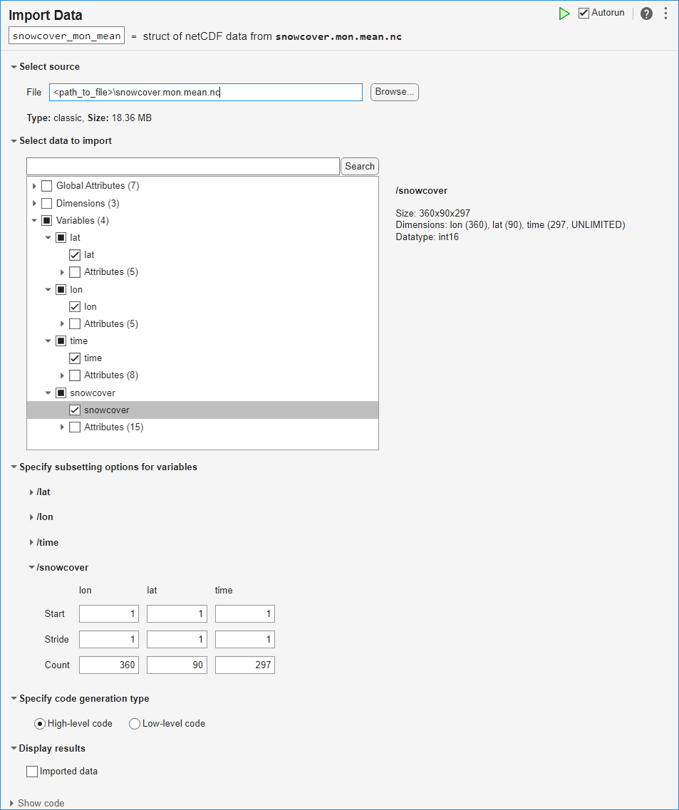
To see the code that this task generates, expand the task display by clicking Show code at the bottom of the task parameter area.
% Create a structure to store imported netCDF data
snowcover_mon_mean = struct();

filename = "snowcover.mon.mean.nc";
snowcover_mon_mean.Variables(1).Name = "lat";
snowcover_mon_mean.Variables(2).Name = "lon";
snowcover_mon_mean.Variables(3).Name = "time";
snowcover_mon_mean.Variables(4).Name = "snowcover";

snowcover_mon_mean.Variables(1).Value = ncread(filename, "/lat");

snowcover_mon_mean.Variables(2).Value = ncread(filename, "/lon");

snowcover_mon_mean.Variables(3).Value = ncread(filename, "/time");

snowcover_mon_mean.Variables(4).Value = ncread(filename, "/snowcover");

clear filename
Organize and Prepare Data
Make local variables for each of the variables from the dataset.
lats = snowcover_mon_mean.Variables(1).Value;
lons = snowcover_mon_mean.Variables(2).Value;
times = snowcover_mon_mean.Variables(3).Value;
snows = snowcover_mon_mean.Variables(4).Value;
Make display versions of lats and lons to prepare for plotting the data. Choose a display scale that shows ten labels on each axis.
numLabels = 10;

latDisps = strings(length(lats),1);
latsLabelInterval = length(lats)/numLabels;
latLabelInds = latsLabelInterval:latsLabelInterval:length(lats);
latDisps(latLabelInds) = lats(latLabelInds);

lonDisps = strings(length(lons),1);
lonsLabelInterval = length(lons)/numLabels;
lonLabelInds = lonsLabelInterval:lonsLabelInterval:length(lons);
lonDisps(lonLabelInds) = lons(lonLabelInds);
The units attribute of the time variable indicates that time is measured in hours since the beginning of the year 1800. Further, the long_name attribute of the snowcover variable indicates that the values are monthly means. Use this information to convert the times vector into corresponding datetime values and also to make a display version of times that includes the month and year but suppresses the day.
sampTimes = datetime("1800-01-01 00:00:00") + hours(times);
sampTimes.Format = "MMM-yyyy";
sampTimeDisps = string(sampTimes);
The first dimension of snows represents a latitude and the second a longitude. To make a heatmap of this data, the first dimension should correspond to a column (longitude) and the second to a row (latitude). Permute these two dimensions of snows.
snows = permute(snows,[2 1 3]);
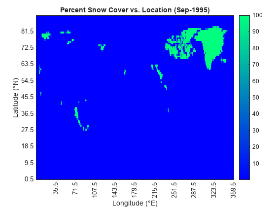
Plot Data
Create a heatmap for the first month of data.
h = heatmap(lons,lats,snows(:,:,1));
h.XLabel = "Longitude (°E)";
h.YLabel = "Latitude (°N)";
h.XDisplayLabels = lonDisps;
h.YDisplayLabels = latDisps;
h.Colormap = winter;
h.GridVisible = "off";
Animate the heatmap by looping through the data for all available times.
for i = 1:numel(sampTimeDisps)
    h.ColorData = snows(:,:,i);
    h.Title = "Percent Snow Cover vs. Location (" + sampTimeDisps(i) + ")";
    pause(0.1)
end
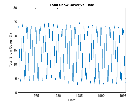
Find Time of Maximum Snow Cover
Compute and plot the total snow cover as a function of time.
cumSnowsbyTime = squeeze(sum(snows,[1 2])) / (length(lats)*length(lons));

plot(sampTimes,cumSnowsbyTime)
xlabel("Date")
ylabel("Total Snow Cover (%)")
title("Total Snow Cover vs. Date")
Find and plot the time of maximum snow cover.
[maxSnowsbyTime,maxSnowsbyTimeInd] = max(cumSnowsbyTime);

h = heatmap(lons,lats,snows(:,:,maxSnowsbyTimeInd));
h.XLabel = "Longitude (°E)";
h.YLabel = "Latitude (°N)";
h.Title = "Percent Snow Cover vs. Location (" + sampTimeDisps(maxSnowsbyTimeInd) + ")";
h.XDisplayLabels = lonDisps;
h.YDisplayLabels = latDisps;
h.Colormap = winter;
h.GridVisible = "off";
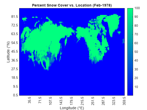
The month of maximal snow cover was February 1978.
Find Locations of Maximum Snow Cover
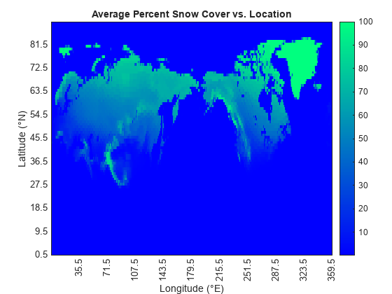
Compute and plot the average snow cover as a function of location.
cumSnowsbyLoc = sum(snows,3) / length(times);

h = heatmap(lons,lats,cumSnowsbyLoc);
h.XLabel = "Longitude (°E)";
h.YLabel = "Latitude (°N)";
h.Title = "Average Percent Snow Cover vs. Location";
h.XDisplayLabels = lonDisps;
h.YDisplayLabels = latDisps;
h.Colormap = winter;
h.GridVisible = "off";
Find and plot the locations of maximum snow cover.
maxSnowsbyLocVal = max(cumSnowsbyLoc,[],"all");
maxSnowsbyLoc = maxSnowsbyLocVal*(cumSnowsbyLoc == maxSnowsbyLocVal);

h = heatmap(lons,lats,maxSnowsbyLoc);
h.XLabel = "Longitude (°E)";
h.YLabel = "Latitude (°N)";
h.Title = "Locations of Maximum Snow Cover";
h.XDisplayLabels = lonDisps;
h.YDisplayLabels = latDisps;
h.Colormap = winter;
h.GridVisible = "off";
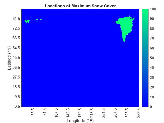
The locations of maximum snow cover include most of Greenland, and parts of Svalbard and Franz Josef Land.
Credits
NH Ease-Grid Snow Cover data provided by the NOAA PSL, Boulder, Colorado, USA, from their website at https://psl.noaa.gov.