Choose Sample Time and Horizons

Sample Time

Duration

Recommended practice is to choose the control interval duration (controller property T_s) initially, and then hold it constant as you tune other controller parameters. If it becomes obvious that the original choice was poor, you can revise T_s. If you do so, you might then need to retune other settings.

Qualitatively, as T_s decreases, rejection of unknown disturbance usually improves and then plateaus. The T_s value at which performance plateaus depends on the plant dynamic characteristics.

However, as T_s becomes small, the computational effort increases dramatically. Thus, the optimal choice is a balance of performance and computational effort.

In Model Predictive Control, the prediction horizon, p is also an important consideration. If one chooses to hold the prediction horizon duration (the product p*T_s) constant, p must vary inversely with T_s. Many array sizes are proportional to p. Thus, as p increases, the controller memory requirements and QP solution time increase.

Consider the following when choosing T_s:

• As a rough guideline, set T_s between 10% and 25% of your minimum desired closed-loop response time.

• Run at least one simulation to see whether unmeasured disturbance rejection improves significantly when T_s is halved. If so, consider revising T_s.

• For process control, T_s >> 1 s is common, especially when MPC supervises lower-level single-loop controllers. Other applications, such as automotive or aerospace, can require T_s < 1 s. If the time needed for solving the QP in real time exceeds the desired control interval, consider the Explicit MPC option.

• For plants with delays, the number of state variables needed for modeling delays is inversely proportional to T_s.

• For open-loop unstable plants, if p*T_s is too large, such that the plant step responses become infinite during this amount of time, key parameters needed for MPC calculations become undefined, generating an error message.

Units

The controller inherits its time unit from the plant model. Specifically, the controller uses the TimeUnit property of the plant model LTI object. This property defaults to seconds.

Prediction Horizon

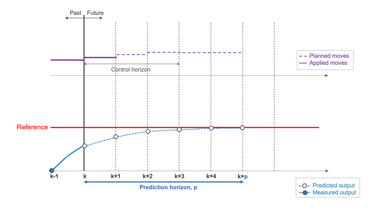
Suppose that the current control interval is k. The prediction horizon, p, is the number of future control intervals the MPC controller must evaluate by prediction when optimizing its MVs at control interval k.

Tips

• Recommended practice is to choose p early in the controller design and then hold it constant while tuning other controller settings, such as the cost function weights. In other words, do not use p adjustments for controller tuning. Rather, the value of p should be such that the controller is internally stable and anticipates constraint violations early enough to allow corrective action.

• If the desired closed-loop response time is T and the control interval is T_s, try p such that T ≈ pT_s.

• Plant delays impose a lower bound on the possible closed-loop response times. Choose p accordingly. To check for a violation of this condition, use the review command.

• Recommended practice is to increase p until further increases have a minor impact on performance. If the plant is open-loop unstable, the maximum p is the number of control intervals required for the open-loop step response of the plant to become infinite. p > 50 is rarely necessary unless T_s is too small.

• Unfavorable plant characteristics combined with a small p can generate an internally unstable controller. To check for this condition, use the review command, and increase p if possible. If p is already large, consider the following:

  • Increase T_s.

  • Increase the cost function weights on MV increments.

  • Modify the control horizon or use MV blocking (see Manipulated Variable Blocking).

  • Use a small p with terminal weighting to approximate LQR behavior (See Terminal Weights and Constraints).

Control Horizon

The control horizon, m, is the number of MV moves to be optimized at control interval k. The control horizon falls between 1 and the prediction horizon p. The default is m = 2. Regardless of your choice for m, when the controller operates, the optimized MV move at the beginning of the horizon is used and any others are discarded. The following picture shows an example in which the control horizon (upper part) is shorter than the prediction horizon (lower part).

MPC signals and horizons

Tips

Reasons to keep m << p are as follows:

• A small m means fewer variables to compute in the QP solved at each control interval, which promotes faster computations.

• If the plant includes delays, m < p is essential. Otherwise, some MV moves might not affect any of the plant outputs before the end of the prediction horizon, leading to a singular QP Hessian matrix. To check for a violation of this condition, use the review command.

• A small m promotes (but does not guarantee) an internally stable controller. Note that manipulated variable blocking can be a more flexible alternative to the simpler control horizon concept. For more information, see Manipulated Variable Blocking.

Defining Sample Time and Horizons

You can define the sample time, prediction horizon, and control horizon when creating an mpc controller at the command line. After creating a controller, mpcobj, you can modify the sample time and horizons by setting the following controller properties:

• Sample time — mpcobj.Ts

• Prediction horizon — mpcobj.p

• Control horizon — mpcobj.m

Also, when designing an MPC controller using MPC Designer, in the Tuning tab, in the Horizon section, you can modify the sample time and horizons.