Magnetic Field in Two-Pole Electric Motor: PDE Modeler App
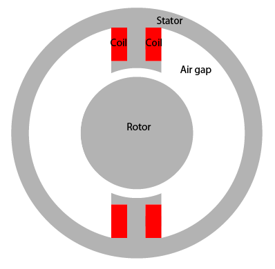
Find the static magnetic field induced by the stator windings in a two-pole electric motor. The example uses the PDE Modeler app. Assuming that the motor is long and end effects are negligible, you can use a 2-D model. The geometry consists of three regions:
Two ferromagnetic pieces: the stator and the rotor (transformer steel)
The air gap between the stator and the rotor
The armature copper coil carrying the DC current
Magnetic permeability of the air and copper is close to the magnetic permeability of a vacuum, μ0 = 4π*10-7 H/m. In this example, use the magnetic permeability μ = μ0 for both the air gap and copper coil. For the stator and the rotor, μ is
where µmax = 5000, µmin = 200, and c = 0.05. The current density J is 0 everywhere except in the coil, where it is 10 A/m2.
The geometry of the problem makes the magnetic vector potential A symmetric with respect to y and antisymmetric with respect to x. Therefore, you can limit the domain to x ≥ 0, y ≥ 0 with the Neumann boundary condition
on the x-axis and the Dirichlet boundary condition A = 0 on the y-axis. Because the field outside the motor is negligible, you can use the Dirichlet boundary condition A = 0 on the exterior boundary.
To solve this problem in the PDE Modeler app, follow these steps:
Set the x-axis limits to
[-1.5
1.5]
and the y-axis limits to[-1 1]. To do this, select Options > Axes Limits and set the corresponding ranges.Set the application mode to Magnetostatics.
Create the geometry. The geometry of this electric motor is complex. The model is a union of five circles and two rectangles. The reduction to the first quadrant is achieved by intersection with a square. To draw the geometry, enter the following commands in the MATLAB® Command Window:
pdecirc(0,0,1,'C1')
pdecirc(0,0,0.8,'C2')
pdecirc(0,0,0.6,'C3')
pdecirc(0,0,0.5,'C4')
pdecirc(0,0,0.4,'C5')
pderect([-0.2 0.2 0.2 0.9],'R1')
pderect([-0.1 0.1 0.2 0.9],'R2')
pderect([0 1 0 1],'SQ1')
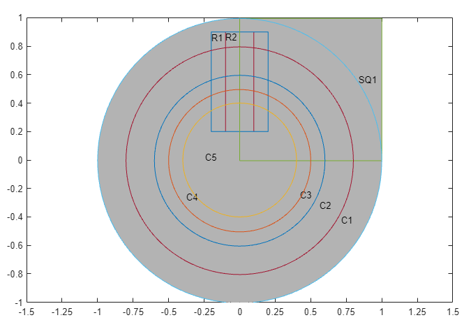
Reduce the model to the first quadrant. To do this, enter
(C1+C2+C3+C4+C5+R1+R2)*SQ1in the Set formula field.Remove unnecessary subdomain borders. To do this, switch to the boundary mode by selecting Boundary > Boundary Mode. Using Shift+click, select borders, and then select Boundary > Remove Subdomain Border until the geometry consists of four subdomains: the rotor (subdomain 1), the stator (subdomain 2), the air gap (subdomain 3), and the coil (subdomain 4). The numbering of your subdomains can differ. If you do not see the numbers, select Boundary > Show Subdomain Labels.
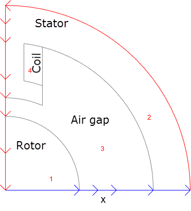
Specify the boundary conditions. To do this, select the boundaries along the x-axis. Select Boundary > Specify Boundary Conditions. In the resulting dialog box, specify a Neumann boundary condition with g = 0 and q = 0.
All other boundaries have a Dirichlet boundary condition with h = 1 and r = 0, which is the default boundary condition in the PDE Modeler app.
Specify the coefficients by selecting PDE > PDE Specification or clicking the
 button on the toolbar.
Double-click each subdomain and specify the following
coefficients:
button on the toolbar.
Double-click each subdomain and specify the following
coefficients:Coil: µ =
4*pi*10^(-7)H/m,J = 10A/m2.Stator and rotor: µ =
4*pi*10^(-7)*(5000./(1+0.05*(ux.^2+uy.^2))+200)H/m, whereux.^2+uy.^2equals to |∇A |2,J = 0(no current).Air gap: µ =
4*pi*10^(-7)H/m,J = 0.
Initialize the mesh by selecting Mesh > Initialize Mesh.
Refine the mesh by selecting Mesh > Refine Mesh.
Choose the nonlinear solver. To do this, select Solve > Parameters and check Use nonlinear solver. Here, you also can adjust the tolerance parameter and choose to use the adaptive solver together with the nonlinear solver.
Solve the PDE by selecting Solve > Solve PDE or clicking the
 button on the toolbar.
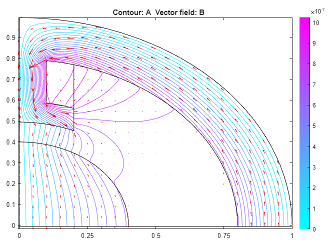
Plot the magnetic flux density B using arrows and the equipotential lines of the magnetostatic potential A using a contour plot. To do this, select Plot > Parameters and choose the contour and arrows plots in the resulting dialog box. Select Plot in x-y grid.
Using Options > Axes Limits, adjust the axes limits as needed. For example, use the Auto check box.
The plot shows that the magnetic flux is parallel to the equipotential lines of the magnetostatic potential.