Thermal Analysis of Disc Brake
This example analyses the temperature distribution of a disc brake. Disc brakes absorb the translational mechanical energy through friction and transform it into the thermal energy, which then dissipates. The transient thermal analysis of a disc brake is critical because the friction and braking performance decreases at high temperatures. Therefore, disc brakes must not exceed a given temperature limit during operation.
This example simulates the disc behavior in two steps:
Perform a highly detailed simulation of the brake pad moving around the disc. Because the computational cost is high, this part of the example only simulates one half revolution (25 ms).
Simulate full braking when the car goes from 100 km/h to 0 km/h in 2.75 seconds, and then remains stopped for 2.25 more seconds in order to allow the heat in the disc to dissipate.
The example uses a vehicle model in Simscape™ Driveline™ to obtain the time dependency of the dissipated power.
Point Heat Source Moving Around the Disc
Simulate a circular brake pad moving around the disc. This detailed simulation over a short timescale models the heat source as a point moving around the disc.
Create an femodel object for transient thermal analysis and include the disc geometry into the model.
model = femodel(AnalysisType="thermalTransient", ...
                Geometry="brake_disc.stl");
Plot the geometry with the face labels.
figure
pdegplot(model,FaceLabels="on");
view([-5 -47])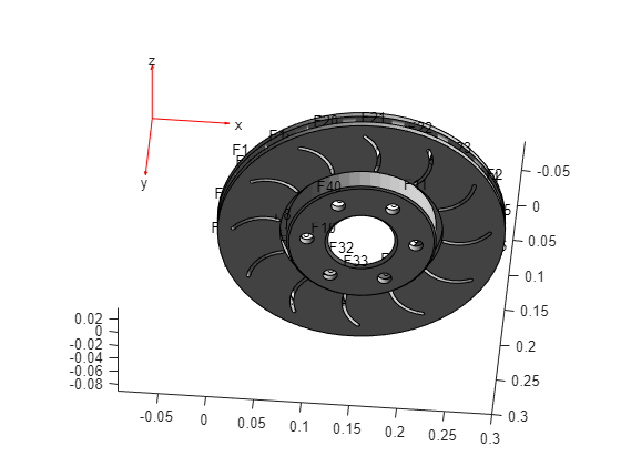
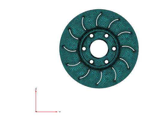
Generate a fine mesh with a small target maximum element edge length. The resulting mesh has more than 130000 nodes (degrees of freedom).
model = generateMesh(model,Hmax=0.005);
Plot the mesh.
pdemesh(model)
view([0,90])
Specify the thermal properties of the material.
model.MaterialProperties = ...
    materialProperties(ThermalConductivity=100, ...
                       MassDensity=8000, ...
                       SpecificHeat=500);
Specify the boundary conditions. All the faces are exposed to air, so there will be free convection.
model.FaceLoad(1:model.Geometry.NumFaces) = ...
    faceLoad(ConvectionCoefficient=10,AmbientTemperature=30);
Model the moving heat source by using a function handle that defines the thermal load as a function of space and time. For the definition of the movingHeatSource function, see the Heat Source Functions section at the bottom of this page.
model.FaceLoad(11) = faceLoad(Heat=@movingHeatSource);
model.FaceLoad(4) = faceLoad(Heat=@movingHeatSource);
Specify the initial temperature.
model.CellIC = cellIC(Temperature=30);
Solve the model for the time steps from 0 to 25 ms.
tlist = linspace(0,0.025,100); % Half revolution
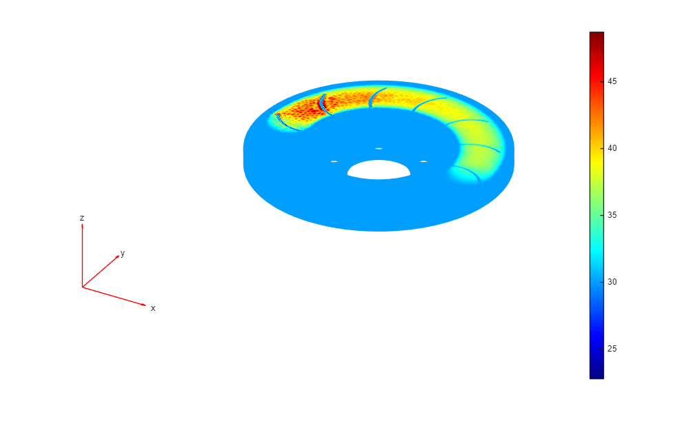
R1 = solve(model,tlist);Plot the temperature distribution at 25 ms.
figure("units","normalized","outerposition",[0 0 1 1])
pdeplot3D(R1.Mesh,ColorMapData=R1.Temperature(:,end))
The animation function visualizes the solution for all time steps. To play the animation, use this command:
animation(model,R1)
Because the heat diffusion time is much longer than the period of a revolution, you can simplify the heat source for the long simulation.
Static Ring Heat Source
Now find the disc temperatures for a longer period of time. Because the heat does not have time to diffuse during a revolution, it is reasonable to approximate the heat source with a static heat source in the shape of the path of the brake pad.
Compute the heat flow applied to the disc as a function of time. To do this, use a Simscape Driveline™ model of a four-wheeled, 2000 kg vehicle that brakes from 100 km/h to 0 km/h in approximately 2.75 s.
driveline_model = "DrivelineVehicle_isothermal";
open_system(driveline_model);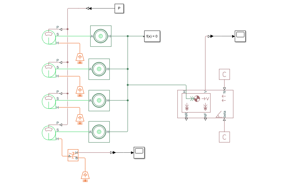
M = 2000; % kg
V0 = 27.8; % m/s, which is around 100 km/h
P = 277; % bar

simOut = sim(driveline_model);

heatFlow = simOut.simlog.Heat_Flow_Rate_Sensor.Q.series.values;
tout = simOut.tout;
Obtain the time-dependent heat flow by using the results from the Simscape Driveline model.
drvln = struct();
drvln.tout = tout;
drvln.heatFlow = heatFlow;
Generate a mesh.
model = generateMesh(model);
Specify the boundary condition as a function handle. For the definition of the ringHeatSource function, see the Heat Source Functions section at the bottom of this page.
model.FaceLoad(11) = faceLoad(Heat=@(r,s)ringHeatSource(r,s,drvln));
model.FaceLoad(4) = faceLoad(Heat=@(r,s)ringHeatSource(r,s,drvln));
Solve the model for times from 0 to 5 seconds.
tlist = linspace(0,5,250);
R2 = solve(model,tlist);
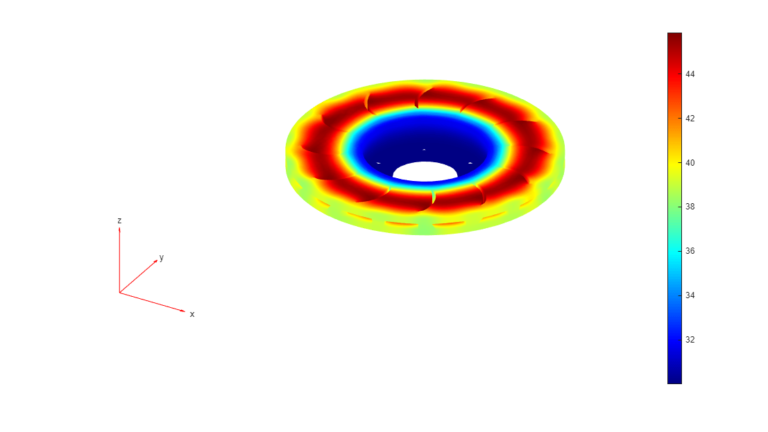
Plot the temperature distribution at the final time step t = 5 seconds.
figure("units","normalized","outerposition",[0 0 1 1])
pdeplot3D(R2.Mesh,ColorMapData=R2.Temperature(:,end))
The animation function visualizes the solution for all time steps. To play the animation, use the following command:
animation(model,R2)
Find the maximum temperature of the disc. The maximum temperature is low enough to ensure that the braking pad performs as expected.
Tmax = max(max(R2.Temperature))
Tmax =
52.2678
Heat Source Functions for Moving and Static Heat Sources
function F = movingHeatSource(region,state)

% Parameters ---------

R = 0.115; % Distance from center of disc to center of braking pad
r = 0.025; % Radius of braking pad
xc = 0.15; % x-coordinate of center of disc
yc = 0.15; % y-coordinate of center of disc

T = 0.05; % Period of 1 revolution of disc

power = 35000; % Braking power in watts
Tambient = 30; % Ambient temperature (for convection)
h = 10; % Convection heat transfer coefficient in W/m^2*K
%--------------------

theta = 2*pi/T*state.time;

xs = xc + R*cos(theta);
ys = yc + R*sin(theta);

x = region.x;
y = region.y;

F = h*(Tambient - state.u); % Convection


if isnan(state.time)
    F = nan(1,numel(x));
end

idx = (x - xs).^2 + (y - ys).^2 <= r^2;

F(1,idx) = 0.5*power/(pi*r.^2);  % 0.5 because there are 2 faces

end
function F = ringHeatSource(region,state,driveline)

% Parameters ---------

R = 0.115; % Distance from center of disc to center of braking pad
r = 0.025; % Radius of braking pad
xc = 0.15; % x-coordinate of center of disc
yc = 0.15; % y-coordinate of center of disc

% Braking power in watts
power = interp1(driveline.tout,driveline.heatFlow,state.time);
Tambient = 30; % Ambient temperature (for convection)
h = 10; % Convection heat transfer coefficient in W/m^2*K
Tf = 2.5; % Time in seconds
%--------------------


x = region.x;
y = region.y;

F = h*(Tambient - state.u); % Convection

if isnan(state.time)
    F = nan(1,numel(x));
end


if state.time < Tf
    rad = sqrt((x - xc).^2 + (y - yc).^2);

    idx = rad >= R-r & rad <= R+r;

    area = pi*( (R+r)^2 - (R-r)^2 );
    F(1,idx) = 0.5*power/area;  % 0.5 because there are 2 faces
end

end