Modeling a Wideband Monostatic Radar in a Multipath Environment
This example shows how to simulate a wideband radar system. A radar system is typically considered to be wideband when its bandwidth exceeds 5% of the system's center frequency. For this example, a bandwidth of 10% will be used.
Exploring the Example
This example expands on the narrowband monostatic radar system explored in the Simulating Test Signals for a Radar Receiver in Simulink example by modifying it for wideband radar simulation. For wideband signals, both propagation losses and target RCS can vary considerably across the system's bandwidth. It is for this reason that narrowband models cannot be used, as they only model propagation and target reflections at a single frequency. Instead, wideband models divide the system's bandwidth into multiple subbands. Each subband is then modeled as a narrowband signal and the received signals within each subband are recombined to determine the response across the entire system's bandwidth.

The model consists of a transceiver, a channel, and a target. The blocks that correspond to each section of the model are:
Transceiver
Linear FM- Creates linear FM pulses.Transmitter- Amplifies the pulses and sends a Transmit/Receive status to theReceiver Preampblock to indicate if it is transmitting.Receiver Preamp- Receives the propagated pulses when the transmitter is off. This block also adds noise to the signal.Platform- Used to model the radar's motion.Signal Processing- Subsystem performs stretch processing, Doppler processing, and noise floor estimation.Matrix Viewer- Displays the processed pulses as a function of the measured range, radial speed, and estimated signal power to interference plus noise power ratio (SINR).
Signal Processing Subsystem

Stretch Processor- Dechirps the received signal by mixing it in the analog domain with the transmitted linear FM waveform delayed to a selected reference range. A more detailed discussion on stretch processing is available in the FMCW Range Estimation example.Decimator- Subsystem models the sample rate of the analog-to-digital converter (ADC) by reducing the simulation's sample rate according to the bandwidth required by the range span selected in the stretch processor.Buffer CPI- Subsystem collects multiple pulse repetition intervals (PRIs) to form a coherent processing interval (CPI), enabling radial speed estimation through Doppler processing.Range-Doppler Response- Computes DFTs along the range and Doppler dimensions to estimate the range and radial speed of the received pulses.CA CFAR 2-D- Estimates the noise floor of the received signals using the cell-averaging (CA) method in both range and Doppler.Compute SINR- Subsystem normalizes the received signal using the CFAR detector's computed threshold, returning the estimated SINR in decibels (dB).
Channel
Wideband Two-Ray- Applies propagation delays, losses, Doppler shifts and multipath reflections off of a flat ground to the pulses. One block is used for the transmitted pulses and another one for the reflected pulses. TheWideband Two-Rayblocks require the positions and velocities of the radar and the target. Those are supplied using theGotoandFromblocks.
Target Subsystem
The Target subsystem models the target's motion and reflects the pulses according to the wideband RCS model and the target's aspect angle presented to the radar. In this example, the target is positioned 3000 meters from the wideband radar and is moving away from the radar at 100 m/s.

Platform- Used to model the target's motion. The target's position and velocity values are used by theWideband Two-Ray Channelblocks to model propagation and by theRange Angleblock to compute the signal's incident angles at the target's location.Range Angle- Computes the propagated signal's incident angles in azimuth and elevation at the target's location.Wideband Backscatter Target- Models the wideband reflections of the target to the incident pulses. The extended wideband target model introduced in the Modeling Target Radar Cross Section example is used for this simulation.
Exploring the Model
Several dialog parameters of the model are calculated by the helper function helperslexWidebandMonostaticRadarParam. To open the function from the model, click on Modify Simulation Parameters block. This function is executed once when the model is loaded. It exports to the workspace a structure whose fields are referenced by the dialogs. To modify any parameters, either change the values in the structure at the command prompt or edit the helper function and rerun it to update the parameter structure.
Results and Displays
The figure below shows the range and radial speed of the target. Target range is computed from the round-trip delay of the reflected pulses. The target's radial speed is estimated by using the DFT to compare the phase progression of the received target returns across the coherent pulse interval (CPI). The target's range and radial speed are measured from the peak of the stretch and Doppler processed output.

Although only a single target was modeled in this example, three target returns are observed in the upper right-hand portion of the figure. The multipath reflections along the transmit and receive paths give rise to the second and third target returns, often referred to as the single- and double-bounce returns respectively. The expected range and radial speed for the target is computed from the simulation parameters.
tgtRange = rangeangle(paramWidebandRadar.targetPos,...
  paramWidebandRadar.sensorPos)
tgtRange =

        3000
tgtSpeed = radialspeed(...
  paramWidebandRadar.targetPos,paramWidebandRadar.targetVel,...
  paramWidebandRadar.sensorPos,paramWidebandRadar.sensorVel)
tgtSpeed =

  -100
This expected range and radial speed are consistent with the simulated results in the figure above.
The expected separation between the multipath returns can also be found. The figure below illustrates the line-of-sight  and reflected path
  geometries.

The modeled geometric parameters for this simulation are defined as follows.
zr = paramWidebandRadar.targetPos(3);
zs = paramWidebandRadar.sensorPos(3);
Rlos = tgtRange;
The length of each of these paths is easily derived.
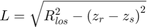
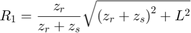

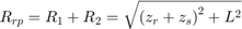
Using these results, the reflected path range can be computed.
L = sqrt(Rlos^2-(zr-zs)^2);
Rrp = sqrt((zs+zr)^2+L^2)
Rrp =

   3.0067e+03
For a monostatic system, the single bounce return can traverse two different paths.
Radar
 Target
  Radar
RadarRadar
Target Radar
In both cases, the same range will be observed by the radar.
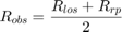
The range separation between all of the multipath returns is then found to be the difference between the observed and line-of-sight ranges.
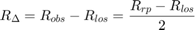
Rdelta = (Rrp-Rlos)/2
Rdelta =

    3.3296
Which matches the multipath range separation observed in the simulated results.
Summary
This example demonstrated how an end-to-end wideband radar system can be modeled within Simulink®. The variation of propagation losses and target RCS across the system's bandwidth required wideband propagation and target models to be used.
The signal to interference plus noise ratio (SINR) of the received target returns was estimated using the CA CFAR 2-D block. The CFAR estimator used cell-averaging to estimate the noise and interference power in the vicinity of the target returns which enabled calculation of the received signal's SINR.
The target was modeled in a multipath environment using the Wideband Two-Ray Channel, which gave rise to three target returns observed by the radar. These returns correspond to the line-of-sight, single-bounce, and double-bounce paths associated with the two-way signal propagation between the monostatic radar and the target. The simulated separation of the multipath returns in range was shown to match the expected separation computed from the modeled geometry.