Processing Radar Reflections Acquired with the Demorad Radar Sensor Platform
Introduction
This example demonstrates how to process and visualize frequency-modulated continuous-wave (FMCW) echoes acquired via the Demorad Radar Sensor Platform with the Phased Array System Toolbox™. By default, I/Q samples and operating parameters are read from a binary file that is provided with this example. Optionally, the same procedure can be used to transmit, receive, and process FMCW reflections from live I/Q samples with your own Demorad by following the instructions later in the example. Acquiring and processing results in one environment decreases development time and facilitates the rapid prototyping of radar signal processing systems.
Required Hardware and Software
This example requires Phased Array System Toolbox™.
For live processing:
Optionally, Analog Devices® Demorad Radar Sensor Platform (and drivers)
Optionally, Phased Array System Toolbox™ Add-On for Demorad
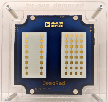
The Analog Devices® Demorad Radar Sensor Platform has an operating frequency of 24 GHz and a maximum bandwidth of 250 MHz. The array on the platform includes 2 transmit elements and 4 receive elements. The receive elements are spaced every half-wavelength of the operating frequency, arranged as a linear array. The transmit elements are also arranged as a linear array and are spaced three half-wavelengths apart. The transmit and receive elements can be seen in the image below.
Installing the Drivers and Add-on
Download the Demorad drivers and MATLAB files from the USB-drive provided by Analog Devices® with the Demorad
Save these to a permanent location on your PC
Add the folder containing the MATLAB files to the MATLAB path permanently
Power up the Demorad and connect to the PC via the Mini-USB port
Navigate to the Device Manager and look for the "BF707 Bulk Device"
Right-click on "BF707 Bulk Device" and select "Update driver"
Select the option "Browse my computer for driver software"
Browse to and select the "drivers" folder from the USB-drive
Install the Phased Array System Toolbox™ Add-On for Demorad from the MATLAB Add-On Manager
Radar Setup and Connection
In this section, we setup the source of the I/Q samples as the default option of the binary file reader. Also contained in this file are the parameters that define the transmitted FMCW chirp, which were written at the time the file was created. If you would like to run this example using live echoes from the Demorad, follow the steps in Installing the Drivers and Add-On and set the "usingHW" flag below to "true". The example will then communicate with the Demorad to transmit an FMCW waveform with the radar operating parameters defined below and send the reflections to MATLAB. The "setup" method below is defined by the object representing the Demorad. "setup" serves both to power on and send parameters to the Demorad.
usingHW = false;  % Set to "true" to use Demorad Radar Sensor Platform

if ~usingHW
  % Read I/Q samples from a recorded binary file
  radarSource = RadarBasebandFileReader('./DemoradExampleIQData.bb',256);
else
  % Instantiate the Demorad Platform interface
  radarSource = DemoradBoard;

  radarSource.SamplesPerFrame = 256;   % Number of samples per frame
  radarSource.AcquisitionTime = 30;    % Length of time to acquire samples (s)

  % Define operating parameters
  radarSource.RampTime = 280e-6;       % Pulse ramp time (s)
  radarSource.PRI = 300e-6;            % Pulse Repetition Interval (s)
  radarSource.StartFrequency = 24e9;   % Pulse start frequency (Hz)
  radarSource.StopFrequency = 24.25e9; % Pulse stop frequency (Hz)
  radarSource.NumChirps = 1;           % Number of pulses to process

  % Establish the connection with the Demorad
  setup(radarSource);
end
Radar Capabilities
Based on the operating parameters defined above, the characteristics of the radar system can be defined for processing and visualizing the reflections. The equations used for calculating the capabilities of the radar system with these operating parameters can be seen below:
Range Resolution
The range resolution (in meters) for a radar with a chirp waveform is defined by the equation
,
where is the bandwidth of the transmitted pulse in Hz:
c0 = physconst('LightSpeed');
wfMetadata = radarSource.Metadata;                % Struct of waveform metadata
bandwidth = wfMetadata.StopFrequency ...
  - wfMetadata.StartFrequency;                    % Chirp bandwidth (Hz)
rangeRes = c0/(2*bandwidth)                       % Range resolution (m)
rangeRes =
0.5996
Maximum Range
The Demorad platform transmits an FMCW pulse as a chirp, or sawtooth waveform. As such, the theoretical maximum range of the radar (in meters) can be calculated using
,
where is the chirp rate. The effective range in practice may vary due to environmental factors such as signal-to-noise ratio (SNR), interference, or size of the testing facility.
kf = bandwidth/wfMetadata.RampTime;          % Chirp rate
maxRange = radarSource.SampleRate*c0/(2*kf)  % Maximum range (m)
maxRange =
158.2904
Beamwidth
The effective beamwidth of the radar board can be approximated by the equation
,
where is the wavelength of the pulse and is the element spacing.
lambda = c0/radarSource.CenterFrequency;               % Signal wavelength (m)
rxElementSpacing = lambda/2;
beamwidth = rad2deg(lambda/ ...
  (radarSource.NumChannels*rxElementSpacing))          % Effective beamwidth (deg)
beamwidth =
28.6479
With a transmit bandwidth of 250 MHz and a 4-element receive array, the range and angular resolution are sufficient to resolve multiple closely spaced objects. The I/Q samples recorded in the binary file are returned from the Demorad platform without any additional digital processing. FMCW reflections received by the Demorad are down-converted to baseband in hardware, decimated, and transferred to MATLAB.
Signal Processing Components
The algorithms used in the signal processing loop are initialized in this section. After receiving the I/Q samples, a 3-pulse canceller removes detections from stationary objects. The output of the 3-pulse canceller is then beamformed and used to calculate the range response. A CFAR detector is used following the range response algorithm to detect any moving targets.
3-Pulse Canceller
The 3-pulse canceller used following the acquisition of the I/Q samples removes any stationary clutter in the environment. The impulse response of a 3-pulse canceller is given as
This equation is implemented in the pulse canceller algorithm defined below.
threePulseCanceller = PulseCanceller('NumPulses',3);Range Response
The algorithms for calculating the range response are initialized below. For beamforming, the sensor array is modeled using the number of antenna elements and the spacing of the receive elements. The sensor array model and the operating frequency of the Demorad are required for the beamforming algorithm. Because the Demorad transmits an FMCW waveform, the range response is calculated using an FFT.
antennaArray = phased.ULA('NumElements',radarSource.NumChannels, ...
  'ElementSpacing',rxElementSpacing);

beamFormer = phased.PhaseShiftBeamformer('SensorArray',antennaArray, ...
'Direction',[0;0],'OperatingFrequency',radarSource.CenterFrequency);

% Setup the algorithm for processing
NFFT = 4096;
rangeResp = phased.RangeResponse( ...
  'DechirpInput', false, ...
  'RangeMethod','FFT', ...
  'ReferenceRangeCentered', false, ...
  'PropagationSpeed',c0, ...
  'SampleRate',radarSource.SampleRate, ...
  'SweepSlope',kf*2, ...
  'RangeFFTLengthSource','Property', ...
  'RangeFFTLength',NFFT, ...
  'RangeWindow', 'Hann');
CFAR Detector
A constant false alarm rate (CFAR) detector is then used to detect any moving targets.
cfar = phased.CFARDetector('NumGuardCells',6,'NumTrainingCells',10);
Scopes
Setup the scopes to view the processed FMCW reflections. We set the viewing window of the range-time intensity scope to 15 seconds.
timespan = 15;

% The Demorad returns data every 128 pulse repetition intervals
rangeScope = phased.RTIScope( ...
  'RangeResolution',maxRange/NFFT,...
  'TimeResolution',wfMetadata.PRI*128, ...
  'TimeSpan', timespan, ...
  'IntensityUnits','power');
Simulation and Visualization
Next, the samples are received from the binary file reader, processed, and shown in the scopes. This loop will continue until all samples are read from the binary file. If using the Demorad, the loop will continue for 30 seconds, defined by the "AcquisitionTime" property of the object that represents the board. Only ranges from 0 to 15 meters are shown, since we have a priori knowledge the target recorded in the binary file is within this range.
while ~isDone(radarSource)
  % Retrieve samples from the I/Q sample source
  x = radarSource();

  % Cancel out any pulses from non-moving objects and beamform
  y = threePulseCanceller(x);
  y = beamFormer(y);

  % Calculate the range response and convert to power
  resp = rangeResp(y);
  rangepow = abs(resp).^2;

  % Use the CFAR detector to detect any moving targets from 0 - 15 meters
  maxViewRange = 15;
  rng_grid = linspace(0,maxRange,NFFT).';
  [~,maxViewIdx] = min(abs(rng_grid - maxViewRange));
  detIdx = false(NFFT,1);
  detIdx(1:maxViewIdx) = cfar(rangepow,1:maxViewIdx);

  % Remove non-detections and set a noise floor at 1/10 of the peak value
  rangepow = rangepow./max(rangepow(:)); % Normalize detections
  noiseFloor = 1e-1;
  rangepow(~detIdx & (rangepow < noiseFloor)) = noiseFloor;

  % Display ranges from 0 - 15 meters in the range-time intensity scope
   rangeScope(rangepow(1:maxViewIdx));
end

The scope shows a single target moving away from the Demorad Radar Sensor Platform until about ~10 meters away, then changing direction again to move back towards the platform. The range-time intensity scope shows the detection ranges.
Summary
This example demonstrates how to interface with the Analog Devices® Demorad Radar Sensor Platform to acquire, process, and visualize radar reflections from live data. This capability enables the rapid prototyping and testing of radar signal processing systems in a single environment, drastically decreasing development time.