Identify Vulnerabilities in DC Microgrids

This example demonstrates how to use reinforcement learning to identify vulnerabilities in cyber-physical systems (CPS) such as a DC microgrid. A DC microgrid (DCmG) is an electric power system that distributes direct current (DC) power within a small geographic area through an interconnected system of distributed generation units (DGU).

Introduction

Cyber-physical systems can have multiple units transmitting or receiving data over a communication network. Cyber attacks on the system might falsify the transmitted data to disrupt the physical system or to financially benefit the attacker.

System operators can build security mechanisms to protect against cyber-attacks, as demonstrated in the example Detect Replay Attacks in DC Microgrids Using Distributed Watermarking (Control System Toolbox). In that example, the two DGUs regulate their voltages and currents against load profiles based on a current consensus rule. The units transmit their sensor measurements to each other over a communication network for the consensus control. An attacker who has gained access to the network might inject a signal $\mathit{a}\left(\mathit{t}\right)$ into the sensor readings to falsify the data. The system is secured by a technique known as watermarking, which adds a periodic signal ${\mathit{w}}_{\mathit{i}}\left(\mathit{t}\right)$ (unknown to the attacker) into the true sensor readings ${\mathit{y}}_{\mathit{i}}\left(\mathit{t}\right)$. The local observer monitors the presence (or absence) of the watermark in the received signals (specifically, the observer removes the watermark signal). Because the watermark is known only to the system operators, any manipulation by an attacker alters the expected pattern of the watermark in the system's output, and operators can detect the cyber-attack.

The diagram below shows the overall architecture of the system.

Identification of System Vulnerabilities

When designing a security mechanism, it might be useful to identify and mitigate any vulnerabilities in the design that can be exploited by attackers. Reinforcement learning provides a testing mechanism for identifying such attacks. Specifically, you can train a policy to attack the system and bypass the existing security measures. If the policy successfully performs the attack without triggering the security measures, analyzing the policy actions can lead to key insights and further improvements of the security measures.

Fix Random Number Stream for Reproducibility

The example code might involve computation of random numbers at various stages. Fixing the random number stream at the beginning of various sections in the example code preserves the random number sequence in the section every time you run it, and increases the likelihood of reproducing the results. For more information, see Results Reproducibility. For more information on controlling the seed used for random number generation, see rng.

previousRngState = rng(0,"twister")

previousRngState = struct with fields:
     Type: 'twister'
     Seed: 0
    State: [625×1 uint32]

The output previousRngState is a structure that contains information about the previous state of the stream. You will restore the state at the end of the example.

DC Microgrid System

The DC microgrid system for this example is modeled in Simulink® and is based on the example Detect Replay Attacks in DC Microgrids Using Distributed Watermarking (Control System Toolbox). First load the system parameters using the dcmgParameters helper Script provided in the example folder.

dcmgParameters

Set the variables that enable (1) or disable (0) the different modes of the system, starting with all modes enabled.

enableAttack = 1;
gaussianAttack = 1;
enableObserver = 1;
enableWatermarking = 1;

Specify the residual and attack limits ${\mathit{r}}_{\max }$ and ${\mathit{a}}_{\max }$.

rmax = 2.0;
amax = 5.0;
attackUpper = amax;
attackLower = -amax;

Open the Simulink model.

mdl = "rldcmicrogrid";
open_system(mdl);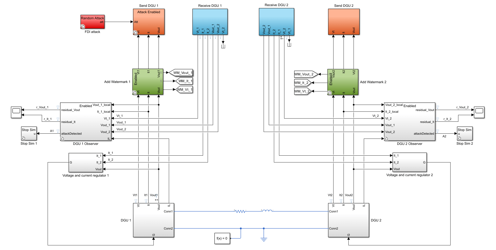

Simulate Under Nominal Conditions

Fix the random stream for reproducibility.

rng(0,"twister");

To simulate the system under no attack, set enableAttack to 0.

enableAttack = 0;

Simulate the model.

nominalOut = sim(mdl);

Visualize the simulation data in the Simulation Data Inspector using the plotInSDI helper function.

plotInSDI(enableAttack)

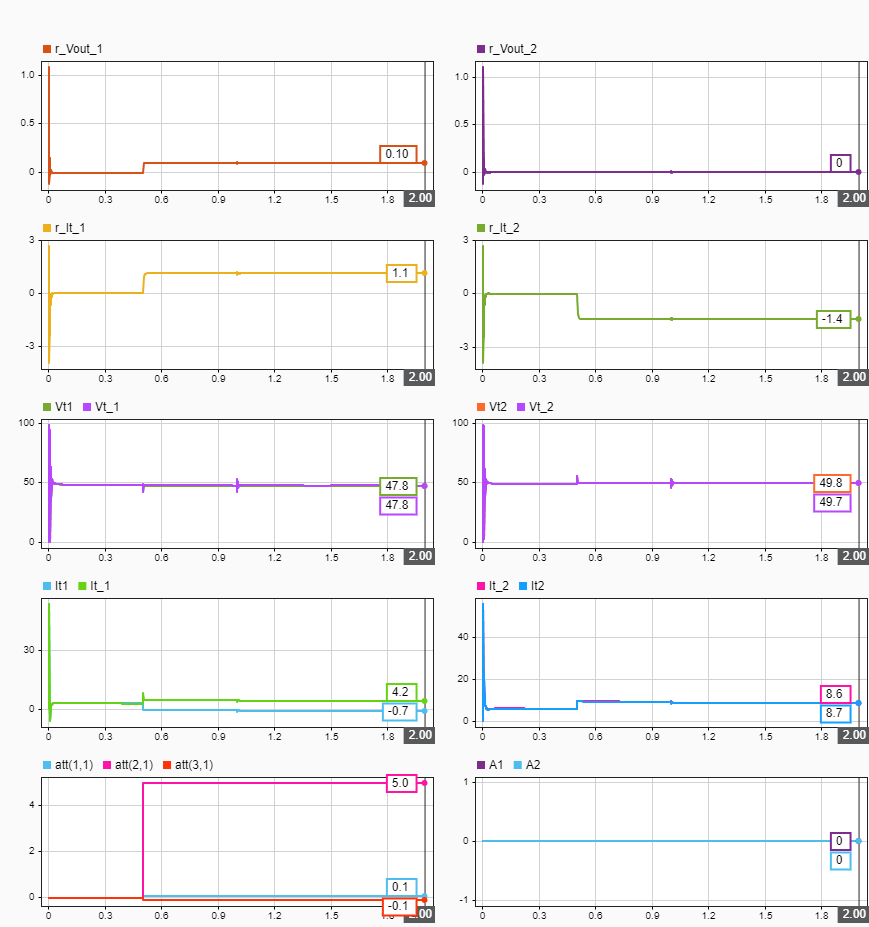
The plots below show the simulation of the various states of the system.

• r_Vout_1 and r_Vout_2 are the voltage residual values for the two DGUs as received over the communication network.

• r_It_1 and r_It_2 are the current residual values as received over the communication network.

• Vt_1, Vt_2, It_1, and It_2 are the voltage and current values as received over the communication network.

• Vt1, Vt2, It1, and It2 are the true voltage and current values.

The system operates as expected under the no attack condition. The voltages and currents satisfy the control requirements and the residual values are zero.

Simulate Gaussian Attack

Simulate the system with an attack model that injects a Gaussian noise into the sensor measurements (${\mathit{Vt}}_1$, ${\mathit{It}}_1$ and ${\mathit{Vout}}_1$) and observe the responses.

Fix the random stream for reproducibility.

rng(0,"twister");

To simulate the Gaussian attack, set enableAttack and gaussianAttack to 1. The attack is saturated within the limits $\pm {\mathit{a}}_{\max }$.

enableAttack = 1;
gaussianAttack = 1;

Simulate the model.

gaussianOut = sim(mdl);

Visualize the simulation data.

plotInSDI(enableAttack)

As shown in the plot, the observer for DGU 1 detects an attack at $\mathit{t}=0.5$ seconds for the attack vector $\mathit{a}\left(\mathit{t}\right)=\left[3.9,2.3,2.3\right]$. At this time, the detection signals A1 and A2 are nonzero because the residual values r_Vout_1 and r_It_1 are greater than ${\mathit{r}}_{\max }$.

Optimal Attack Problem

The optimal attack bypasses the security of the system while satisfying a set of constraints. The attack model represents the following scenario:

• The attack is performed on the data transmitted from the DGU 1 unit, while DGU 2 data remains unaffected (see the diagram of the system architecture earlier in this example).

• The attacker adds a disturbance to the true signals ${\mathit{Vt}}_1$, ${\mathit{It}}_1$ and ${\mathit{Vout}}_1$. This type of attack is known as false data injection (FDI).

• The attack policy aims to find an attack sequence $\mathit{S}=\left[{\mathit{a}}_0,{\mathit{a}}_1,...,{\mathit{a}}_{\mathit{T}}\right]$ for some time horizon $\mathit{T}$ that minimizes the line current ${\mathit{It}}_1$ while being undetected by the observers (${\mathit{r}}_{\mathit{k}}\le {\mathit{r}}_{\max }$). Minimizing the current is one of many possible attack objectives.

• The magnitude of the attack at any time step is kept small (${\mathit{a}}_{\mathit{k}}\le {\mathit{a}}_{\max }$) to avoid detection.

This scenario leads to the constrained optimization problem

$$\underset{\mathit{S}}{\min }\sum _{\mathit{k}=0}^{\mathit{T}}{\mathit{It}}_{1,\mathit{k}}$$

$$\mathit{s}.\mathit{t}.{\mathit{r}}_{\mathit{k}}\le {\mathit{r}}_{\max }\mathrm{and}{\mathit{a}}_{\mathit{k}}\le {\mathit{a}}_{\max }$$

The corresponding unconstrained problem is

$$\underset{\mathit{S}}{\max }\sum _{\mathit{k}=0}^{\mathit{T}}{-\mathit{It}}_{1,\mathit{k}}-\mathit{W}*{\mathit{D}}_{\mathit{k}}\left({\mathit{r}}_{\mathit{k}},{\mathit{a}}_{\mathit{k}},{\mathit{r}}_{\max },{\mathit{a}}_{\max }\right)$$

where ${\mathit{r}}_{\mathit{k}}$, ${\mathit{a}}_{\mathit{k}}$ are the observer residual and attack vectors at time $\mathit{k}$, and $\mathit{W}*{\mathit{D}}_{\mathit{k}}$ is a soft penalty for deviating from the allowable residual and attack limits. You solve this unconstrained problem using reinforcement learning.

Create Environment Object

The first step in solving the unconstrained problem is to create the environment object. The environment is the DC microgrid system under attack. For this environment:

• The observation vector $0.1*\left[{\mathit{Vt}}_1,{\mathit{It}}_1,{\mathit{Vout}}_1,{\mathit{Vt}}_2,{\mathit{It}}_2,{\mathit{Vout}}_2,{\mathit{a}}_{\mathit{last}}\right]$ contains the true voltage and current values from the two DGU units, as well as the attack vector from the last time step scaled by the factor 0.1.

The action is a three-element vector representing the cyber-attack. The attacker adds the action vector to the $\left[{\mathit{Vt}}_1,{\mathit{It}}_1,{\mathit{Vout}}_1\right]$ measurements during the transmission from the DGU 1 unit to the DGU 2 unit.

• The reward at time $\mathit{k}$ is given by:

${\mathit{R}}_{\mathit{k}}={-0.1\mathit{It}}_{1,\mathit{k}}-0.0001{\mathit{D}}_{\mathit{k}}$, where ${\mathit{D}}_{\mathit{k}}$ is a quadratic exterior penalty computed using the exteriorPenalty function.

Disable the Gaussian attack model.

gaussianAttack = 0;

Create the observation and action input specifications.

obsInfo = rlNumericSpec([9,1]);
obsInfo.Name = "observation";

actInfo = rlNumericSpec([3,1]);
actInfo.Name = "action";

Specify the action range [-1,1]. The action is scaled up using attackGain in the Simulink model, and saturated within [attackLower,attackUpper].

actInfo.UpperLimit = 1;
actInfo.LowerLimit = -1;
attackGain = [0.1;10;0.1];

Create the Simulink environment object.

blk = mdl + "/FDI attack/RL Attack/RL/RL Agent"; 
env = rlSimulinkEnv(mdl,blk,obsInfo,actInfo)

env = 
SimulinkEnvWithAgent with properties:

           Model : rldcmicrogrid
      AgentBlock : rldcmicrogrid/FDI attack/RL Attack/RL/RL Agent
        ResetFcn : []
  UseFastRestart : on

Specify a reset function to set the time of attack to 0 at the beginning of the training episodes, so that the agent starts learning when the attack is going on.

env.ResetFcn = @(in) setVariable(in,"timeOfAttack",0);

Create TD3 Agent

The agent in this example is a twin-delayed deep deterministic policy gradient (TD3) agent. TD3 agents use two parameterized Q-value function approximators (that is, two critics) to estimate the value (that is, the expected cumulative long-term reward) of the policy. For more information on TD3 agents, see Twin-Delayed Deep Deterministic (TD3) Policy Gradient Agent.

Create an agent initialization object to initialize the default critic network with the hidden layer size 300.

initOpts = rlAgentInitializationOptions(NumHiddenUnit=300);

Specify the agent options for training using an rlTD3AgentOptions object. For this agent:

• Use an experience buffer with capacity 1e6 to collect experiences. A larger capacity maintains a diverse set of experiences in the buffer.

• Use mini-batches of 300 experiences. Smaller mini-batches are computationally efficient but may introduce variance in training. By contrast, larger batch sizes can make the training stable but require higher memory.

• Specify the learning rate of 1e-5 for the actor and critics. A smaller learning rate can improve the stability of training.

• Specify the initial standard deviation value of 0.2 for the agent's exploration model. The standard deviation decays at the rate of 1e-6 until it reaches the minimum value of 0.01. This decay rate facilitates exploration toward the beginning and exploitation toward the end of training.

• The sample time is ${\mathit{T}}_{\mathit{s}}=5\mathit{e}-5$ seconds.

agentOpts = rlTD3AgentOptions( ...
    SampleTime=Ts, ...
    ExperienceBufferLength=1e6, ...
    MiniBatchSize=300);

agentOpts.ActorOptimizerOptions.LearnRate = 1e-5;
for i = 1:2
    agentOpts.CriticOptimizerOptions(i).LearnRate = 1e-5;
end

agentOpts.ExplorationModel.StandardDeviation = 0.2;
agentOpts.ExplorationModel.StandardDeviationMin = 0.01;
agentOpts.ExplorationModel.StandardDeviationDecayRate = 1e-6;

Create the TD3 agent using the observation and action input specifications, initialization options, and agent options. When you create the agent, the initial parameters of the critic network are initialized with random values. Fix the random number stream so that the agent is always initialized with the same parameter values.

rng(0,"twister");
agent = rlTD3Agent(obsInfo,actInfo,initOpts,agentOpts)

agent = 
  rlTD3Agent with properties:

        ExperienceBuffer: [1×1 rl.replay.rlReplayMemory]
            AgentOptions: [1×1 rl.option.rlTD3AgentOptions]
    UseExplorationPolicy: 0
         ObservationInfo: [1×1 rl.util.rlNumericSpec]
              ActionInfo: [1×1 rl.util.rlNumericSpec]
              SampleTime: 5.0000e-05

Train Agent

To train the agent, first specify the training options. For this example, use the following options:

• Run the training for 50 episodes, with each episode lasting at most ceil(0.1/Ts) time steps.

• Specify an averaging window length of 10 for the episode rewards.

For more information see rlTrainingOptions.

trainOpts = rlTrainingOptions(...
    MaxEpisodes=50, ...
    MaxStepsPerEpisode=floor(0.1/Ts), ...
    ScoreAveragingWindowLength=10, ...
    StopTrainingCriteria="none");

Fix the random stream for reproducibility.

rng(0,"twister");

Enable the attack, and disable the Gaussian attack model.

enableAttack = 1;
gaussianAttack = 0;

Train the agent using the train function. Training this agent is a computationally intensive process that takes several minutes to complete. To save time while running this example, load a pretrained agent by setting doTraining to false. To train the agent yourself, set doTraining to true.

doTraining = false;
if doTraining
    % Train the agent.
    trainResult = train(agent,env,trainOpts);
else
    % Load the pretrained agent for the example.
    load("DCMicrogridAgent.mat","agent");
end

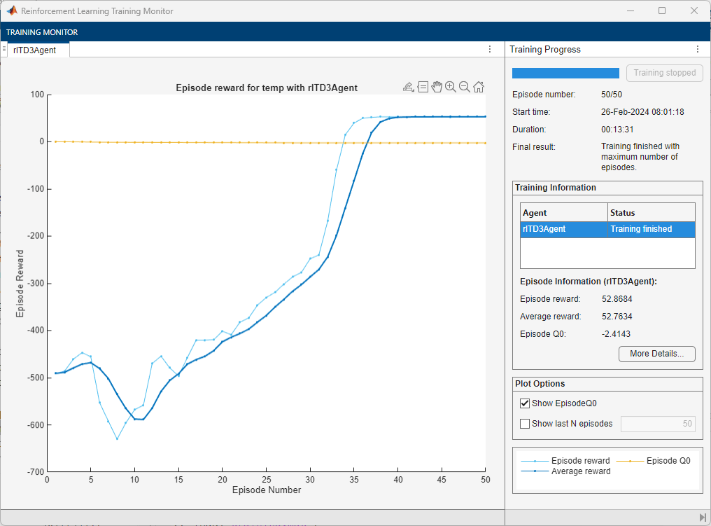
A snapshot of the training progress is shown below. You may expect different results due to randomness in training.

Simulate Learned Attack

Fix the random stream for reproducibility.

rng(0,"twister");

Simulate the model with the trained reinforcement learning agent.

enableAttack = 1;
gaussianAttack = 0;
optimalOut = sim(mdl);

Visualize the simulation data.

plotInSDI(enableAttack)

The optimal attack signal is able to keep the residual values within the allowable range $\pm {\mathit{r}}_{\max }$, while creating impact on the current regulation. At 2.0 seconds, as a result of the attack $\mathit{a}\left(\mathit{t}\right)=\left[0.1,5.0,-0.1\right]$, a false current (It_1) of 4.2 A is transmitted over the network while the true value (It1) is -0.7 A. To satisfy the current consensus rule, the DGU 2 unit compensates by generating a higher current (It_2) than required, creating an advantage for the DGU 1 unit over time.

Analysis and Conclusion

Compare the energy generation of the DGUs for the nominal and optimal attack cases. First, extract the logged data from the simulations.

eNominal(1) = getElement(nominalOut.logsout,"E1");
eNominal(2) = getElement(nominalOut.logsout,"E2");
eOptimal(1) = getElement(optimalOut.logsout,"E1");
eOptimal(2) = getElement(optimalOut.logsout,"E2");
attOptimal  = getElement(optimalOut.logsout,"att");
refLoad(1)  = getElement(optimalOut.logsout,"IL1");
refLoad(2)  = getElement(optimalOut.logsout,"IL2");

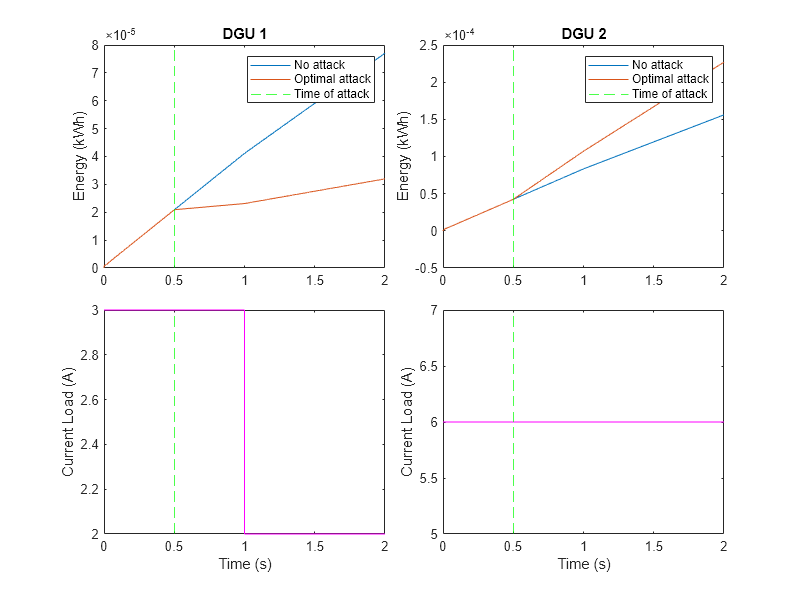
Plot the energy consumption in the two units. At the time of attack (0.5 seconds), the optimal attack policy reduces the energy generation in DGU 1 while simultaneously increasing the generation in DGU 2. The effect continues even after the load change at 1 second.

f = figure();
t = tiledlayout(f,2,2,TileSpacing="compact");
for i = 1:2
    ax = nexttile(t);
    plot(ax,eNominal(i).Values.Time,eNominal(i).Values.Data);
    hold(ax,"on");
    plot(ax,eOptimal(i).Values.Time,eOptimal(i).Values.Data);
    xline(ax,timeOfAttack,"g--");
    ylabel(ax,"Energy (kWh)");
    legend(ax,["No attack","Optimal attack","Time of attack"]);
    title(ax,sprintf("DGU %d",i));
end
for i = 1:2
    ax = nexttile(t);
    plot(ax,refLoad(i).Values.Time,refLoad(i).Values.Data(:),"m");
    hold(ax,"on");
    xline(ax,timeOfAttack,"g--");
    xlabel(ax,"Time (s)");
    ylabel(ax,"Current Load (A)");
end
f.Position(3:4) = [800,600];

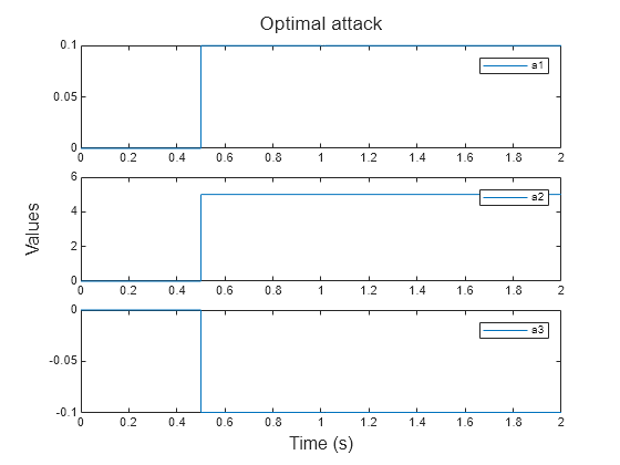
Plot the optimal attack vector over time. The magnitude of attack on the ${\mathit{Vt}}_1$ and ${\mathit{Vout}}_1$ signals ($\mathit{a1}$and $\mathit{a3}$) is low, while the attack on the ${\mathit{It}}_1$ signal ($\mathit{a2}$) is large. The attacker bypasses observer-based security by freely modifying the ${\mathit{It}}_1$ signal. This observation can be used as a starting point to investigate and further improve the system. For instance, the observer design can be improved to consider any difference between the actual and transmitted values of the ${\mathit{It}}_{\mathit{i}}$ signal (out of the scope for this example).

h = figure();
t = tiledlayout(h,3,1,TileSpacing="compact");
for i = 1:3
    ax = nexttile(t);
    plot(ax,attOptimal.Values.Time, ...
        squeeze(attOptimal.Values.Data(i,:,:)));
    legend(ax,"a"+i);
end
title(t,"Optimal attack");
xlabel(t,"Time (s)");
ylabel(t,"Values");

Restore the random number stream using the information stored in previousRngState.

rng(previousRngState);

Helper Functions

function plotInSDI(enableAttack)
% Open and configure the SDI
Simulink.sdi.view;
Simulink.sdi.clearAllSubPlots;
% Generate subplots
if enableAttack
    Simulink.sdi.setSubPlotLayout(5,2);
else
    Simulink.sdi.setSubPlotLayout(4,2);
end
% Get the current run
run = Simulink.sdi.getCurrentSimulationRun("rldcmicrogrid");
% Subplot 1
plotOnSubPlot(getSignalsByName(run,"r_Vout_1"),1,1,true);
% Subplot 2
plotOnSubPlot(getSignalsByName(run,"r_Vout_2"),1,2,true);
% Subplot 3
plotOnSubPlot(getSignalsByName(run,"r_It_1"),2,1,true);
% Subplot 4
plotOnSubPlot(getSignalsByName(run,"r_It_2"),2,2,true);
% Subplot 5
plotOnSubPlot(getSignalsByName(run,"Vt1"),3,1,true);
plotOnSubPlot(getSignalsByName(run,"Vt_1"),3,1,true);
% Subplot 6
plotOnSubPlot(getSignalsByName(run,"Vt2"),3,2,true);
plotOnSubPlot(getSignalsByName(run,"Vt_2"),3,2,true);
% Subplot 7
plotOnSubPlot(getSignalsByName(run,"It1"),4,1,true);
plotOnSubPlot(getSignalsByName(run,"It_1"),4,1,true);
% Subplot 8
plotOnSubPlot(getSignalsByName(run,"It2"),4,2,true);
plotOnSubPlot(getSignalsByName(run,"It_2"),4,2,true);
% Subplots 9 and 10
if enableAttack
    % Subplot 9
    att = getSignalsByName(run,"att");
    plotOnSubPlot(att.Children(1),5,1,true);
    plotOnSubPlot(att.Children(2),5,1,true);
    plotOnSubPlot(att.Children(3),5,1,true);
    % Subplot 10
    plotOnSubPlot(getSignalsByName(run,"A1"),5,2,true);
    plotOnSubPlot(getSignalsByName(run,"A2"),5,2,true);
end
end