Fit S-Parameters with a Rational Function

Step 2 of 5 in Model and Analyze High-Speed Backplanes

This example shows how to use RF Toolbox™ to model a differential high-speed backplane channel using rational functions. This type of model is useful to signal integrity engineers, whose goal is to reliably connect high-speed semiconductor devices with, multi-Gbps serial data streams across backplanes and printed circuit boards.

Compared to traditional techniques such as linear interpolation, rational function fitting provides more insight into the physical characteristics of a high-speed backplane. It provides a means, called model order reduction, of making a trade-off between complexity and accuracy. For a given accuracy, rational functions are less complex than other types of models such as FIR filters generated by IFFT techniques. In addition, rational function models inherently constrain the phase to be zero on extrapolation to DC. Less physically-based methods require elaborate constraint algorithms in order to force the extrapolated phase to zero at DC.

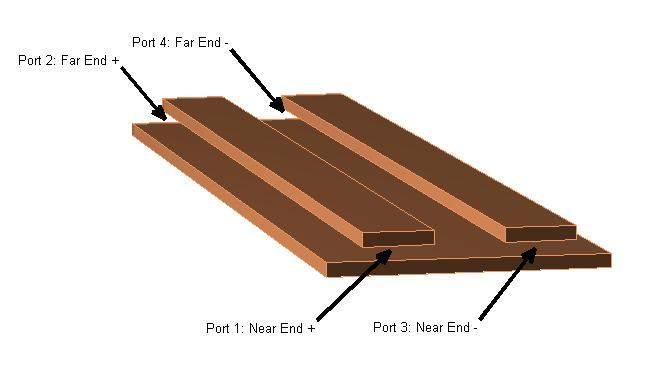
Figure 1: A differential high-speed backplane channel

Read Single-Ended 4-Port S-Parameters and Convert Them to Differential 2-Port S-Parameters

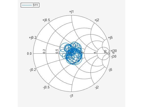
Read a Touchstone® data file, default.s4p, into an sparameters object. The parameters in this data file are the 50-ohm S-parameters of the single-ended 4-port passive circuit shown in Figure 1, at 1496 frequencies ranging from 50 MHz to 15 GHz. Then, get the single-ended 4-port S-parameters and use the matrix conversion function s2sdd to convert them to differential 2-port S-parameters. Finally, plot the differential S11 parameter on a Smith chart.

filename = 'default.s4p';
backplane = sparameters(filename);
data = backplane.Parameters;
freq = backplane.Frequencies;
z0 = backplane.Impedance;

Convert to 2-port differential S-parameters.

diffdata = s2sdd(data);  
diffz0 = 2*z0;

By default, s2sdd expects ports 1 and 3 to be input and ports 2 and 4 to be output. However if your data has ports 1 and 2 as input and ports 3 and 4 as output, then use 2 as the second input argument to s2sdd function to specify this alternate port arrangement. For example, diffdata = s2sdd(data,2);

diffsparams = sparameters(diffdata,freq,diffz0)

diffsparams = 
  sparameters with properties:

      Impedance: 100
       NumPorts: 2
     Parameters: [2x2x1496 double]
    Frequencies: [1496x1 double]

figure
smithplot(diffsparams,1,1)

Compute Transfer Function and Its Rational Function Object Representation

First, use the s2tf function to compute the differential transfer function. Then, use the rational function to compute the analytical form of the transfer function and store it in an object. The rational function fits a rational function object to the specified data over the specified frequencies. The run time depends on the computer, the fitting tolerance, the number of data points, among other factors.

difftransfunc = s2tf(diffdata,diffz0,diffz0,diffz0);
rationalfunc = rational(freq,difftransfunc,Tolerance=-60)

rationalfunc = 
  rational with properties:

      NumPorts: 1
      NumPoles: 386
         Poles: [386x1 double]
      Residues: [1x1x386 double]
    DirectTerm: 0
         ErrDB: -60.9431

npoles = rationalfunc.NumPoles;
fprintf('The derived rational function contains %d poles.\n',npoles);

The derived rational function contains 386 poles.

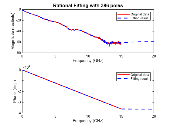
Validate Differential-Mode Frequency Response

Use the freqresp method of the rational object to get the frequency response of the rational function object. Then, create a plot to compare the frequency response of the rational function object and that of the original data.

freqsforresp = linspace(0,20e9,2000)';
resp = freqresp(rationalfunc,freqsforresp);

figure
subplot(2,1,1)
plot(freq*1.e-9,20*log10(abs(difftransfunc)),'r',freqsforresp*1.e-9, ...
                20*log10(abs(resp)),'b--','LineWidth',2)
title(sprintf('Rational Fitting with %d poles',npoles),'FontSize',12)
ylabel('Magnitude (decibels)')
xlabel('Frequency (GHz)')
legend('Original data','Fitting result')

subplot(2,1,2)
origangle = unwrap(angle(difftransfunc))*180/pi;
plotangle = unwrap(angle(resp))*180/pi;
plot(freq*1.e-9,origangle,'r',freqsforresp*1.e-9,plotangle,'b--', ...
    'LineWidth',2)
ylabel('Phase (deg.)')
xlabel('Frequency (GHz)')
legend('Original data','Fitting result')

Calculate and Plot Differential Input and Output Signals of High-Speed Backplane

Generate a random 2 Gbps pulse signal. Then, use the timeresp method of the rational object to compute the response of the rational function object to the random pulse. Finally, plot the input and output signals of the rational function model that represents the differential circuit.

datarate = 2*1e9;                % Data rate: 2 Gbps 
samplespersymb = 100; 
pulsewidth = 1/datarate;            
ts = pulsewidth/samplespersymb;
numsamples = 2^17;
numplotpoints = 10000;

t_in = double((1:numsamples)')*ts;
input = sign(randn(1,ceil(numsamples/samplespersymb)));
input = repmat(input,[samplespersymb, 1]);
input = input(:);
[output,t_out] = timeresp(rationalfunc,input,ts);

figure
subplot(2,1,1)
plot(t_in(1:numplotpoints)*1e9,input(1:numplotpoints),'LineWidth',2)
title([num2str(datarate*1e-9),' Gbps signal'],'FontSize',12)
ylabel('Input signal')
xlabel('Time (ns)')
axis([-inf,inf,-1.5,1.5])

subplot(2,1,2)
plot(t_out(1:numplotpoints)*1e9,output(1:numplotpoints),'LineWidth',2)
ylabel('Output signal')
xlabel('Time (ns)')
axis([-inf,inf,-1.5,1.5])

Plot Eye Diagram of 2 Gbps Output Signal

Estimate and remove the delay from the output signal and create an eye diagram by using Communications Toolbox™ functions.

if ~isempty(which('eyediagram'))
    ignoreBits = 1500;
    eyediagram(output(ignoreBits:end),2*samplespersymb,2/datarate)
end

Related Topics

• Use S-parameters with Port Reduction
• Compute Differential TDR and TDT
• Build Simulink Model from Rational Function

Model and Analyze High-Speed Backplanes

Next