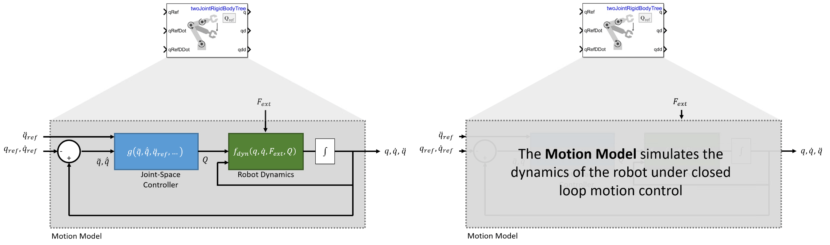
Joint-Space Motion Model
The joint-space motion model characterizes the motion of a manipulator under closed-loop joint-space position control, as used in the jointSpaceMotionModel object and Joint Space Motion Model block.
Robot manipulators are typically position-controlled devices. For joint-space control, you specify the vector of joint angles or positions, , that tracks a reference configuration, . You can do this by using closed-loop control on the robot joints and using the motion model to simulate the behavior of a robot under this control.
For this approach to most closely approximate the motion of the actual system, you must accurately represent the dynamics of the controller and plant. This topic covers the methods of modeling the behavior of the robot under closed-loop joint-space position control:
As a system subject to Computed Torque Control
As a system subject to PD Control
As a system with Independent Joint Motion
Background
Joint-Space vs. Task-Space Motion Models
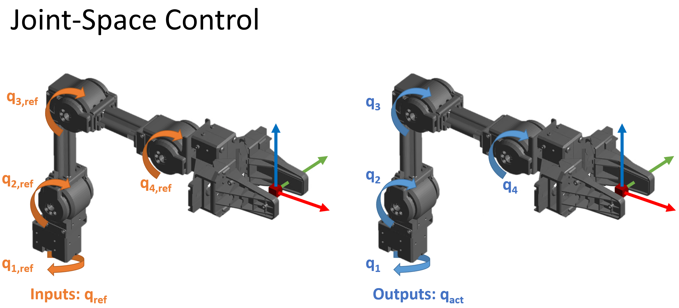
Generally, there are two categories of robot position control:
Joint-Space motion control — In this case, the position input of the robot is specified as a vector of joint angles or positions, known as the robot's joint configuration, . The controller tracks a reference configuration, , and returns the actual joint configuration . This is also known as configuration-space control.
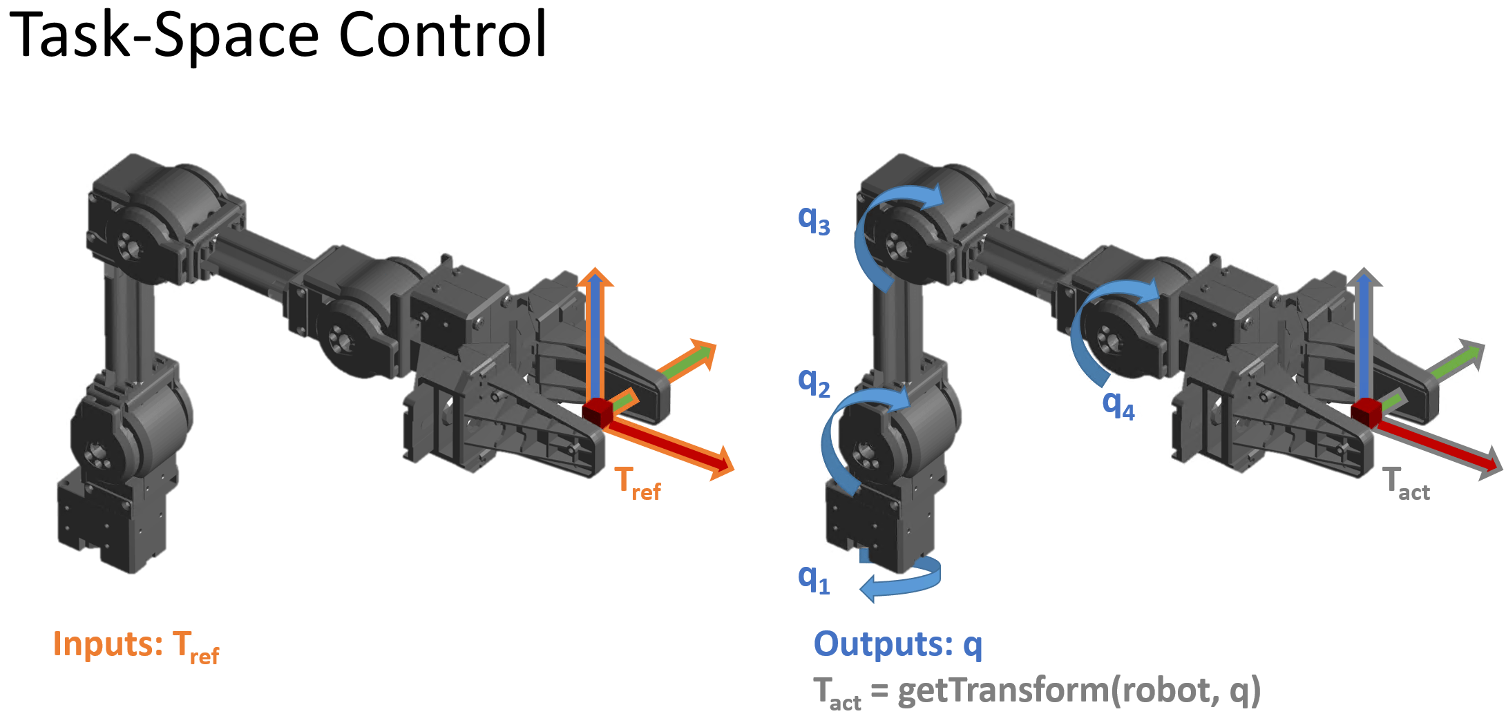
Task-Space motion control — The position is specified to a controller as an end-effector pose. Then the controller drives the robot's joint configurations to the values that move the end effector to the specified pose. This is sometimes referred to as operational-space control.
The following figures shows the different types of inputs/outputs in these two motion control categories.
This topic page is specific to joint-space motion control, as used in the jointSpaceMotionModel object and Joint Space Motion Model block. For task-space motion models, see the taskSpaceMotionModel object. For an example that covers the difference between task-space and joint-space control in greater detail, see Plan and Execute Task- and Joint-Space Trajectories Using Kinova Gen3 Manipulator.
Usage in MATLAB® and Simulink®
The joint-space motion model can be represented in MATLAB or Simulink.
In Simulink, the Joint Space Motion model block accepts the reference inputs and optional external force when applicable, and returns the joint configuration, velocity, and acceleration. The block handles integration, so no additional integration is required.
In MATLAB, the
jointSpaceJointModelsystem object models the closed-loop motion. Thederivativemethod returns derivatives of the joint configuration, velocity, and acceleration at each instant in time, so you must use an ODE solver or equivalent external integration method to simulate the motion in time.
For a more specific overview, refer to the associated documentation pages.
State
The joint-space motion model state consists of these values:
— Robot joint configuration, as a vector of joint positions. Specified in for revolute joints and for prismatic joints.
— Vector of joint velocities in for revolute joints and for prismatic joints
— Vector of joint accelerations in for revolute joints or for prismatic joints
Equations of Motion for the Types of Closed-Loop Joint-Space Motion
The joint-space motion model is used when you need a low-fidelity model of your system under closed-loop control and the inputs are specified as joint configuration, velocity, and acceleration. The motion model includes three ways to model its overall behavior:
As a system under Computed Torque Control — The rigid body dynamics are modeled using the standard rigid body Robot Dynamics, but compensating for the full-body dynamics and assigning error dynamics.
As a system under PD Control — The rigid body dynamics are modeled using the standard rigid body Robot Dynamics with a joint torque input given by proportional-derivative (PD) control and gravity compensation. This model represents a controller that does not compensate tightly for the overall effects of rigid body motion.
As a system with Independent Joint Motion — Each joint is modeled independently as a configuration-invariant closed-loop second-order system. This model is a lower-fidelity model that ignores robot dynamics and assumes a closed loop response. The model may be considered a best-case scenario for how closed-loop motion may behave in the absence of external forces since the dynamics are simplified and directly prescribed.
To set these different motion types, use the MotionType property of the jointSpaceMotionModel object. These motion types are not exhaustive, but they do provide a set of options to use when approximating the closed-loop behavior of your system. For details and suggestions on when to use which model, see the sections below.
In the following sections, the equations of motion for each model are introduced, in order of decreasing complexity. Here, complexity is a measure of how much computation occurs in a given motion model. A high-complexity variation models dynamics subject to a fairly advanced controller by directly simulating the controller and dynamics within the loop, while a low complexity model uses simplified dynamics to represent the overall error behavior.
Notation & Terminology
Many of the equations of motion for the closed-loop system are derived from the standard rigid body Robot Dynamics, which defines the open-loop motion of the robot. Additionally, the equations frequently use a tilde to indicate error dynamics, e.g. .
Computed Torque Control
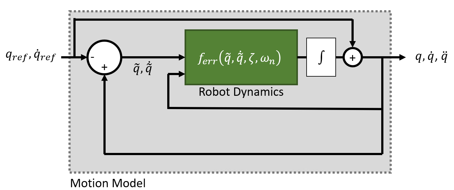
When the motion model is defined as a robot subject to computed torque control, the motion model uses standard rigid body Robot Dynamics, but the generalized force input is given by a control law that compensates for the rigid body dynamics and instead assigns a second-order error dynamics response.
Inputs — This model accepts as the desired reference joint configuration, velocities, and accelerations as vectors. The user may also optional provide a matrix of external forces and torques , specified in Newtons and Newton-meters, generated using the
externalForcefunction.Outputs — The model outputs as the joint configuration, velocities, and accelerations as vectors. In the MATLAB version of the model, only accelerations are returned, and the user must choose an integrator or ODE solver to return the other states.
Complexity — This is high complexity. The motion model uses full rigid body dynamics with optional external forces, the controller is modeled as part of the closed loop system, and the controller includes dynamic compensation terms.
When to apply — Use when the closed-loop system being simulated has approximable error dynamics, or when it uses a controller that treats the robot as a multi-body system, and external forces may be present.
The resultant closed-loop system aims to achieve the following second error behavior for the -th joint:
These parameters characterize the desired response defined for each joint:
— Natural frequency, specified in Hz ()
— The damping ratio, which is unitless
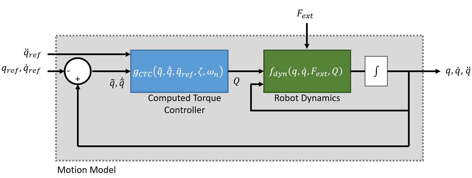
As seen in the diagram, the complete system consists of the standard rigid body robot dynamics with a control law that enforces closed error dynamics via the generalized force input :
where,
— is a joint-space mass matrix based on the current robot configuration Calculate this matrix by using the
massMatrixobject function.— is the Coriolis terms. Together with the joint velocity, this forms the velocity product , which can be calculated using the
velocityProductobject function.— is the torques and forces required for all joints to maintain their positions due to gravitational weights & forces acting on the robot, given the specified Gravity. Calculate the gravity torque by using the
gravityTorqueobject function.— -by- diagonal matrix of natural frequencies in the NaturalFrequency property of the
jointSpaceMotionModelobject are in Hz ().— -by- diagonal matrix of the products of the squared natural frequencies , and damping ratios , specified in the DampingRatio property of the
jointSpaceMotionModelobject.
The values of and may be set directly, or they may be provided using the updateErrorDynamicsFromStep method, which computes values for and based on desired unit step response (defined using the transient behavior characteristics).
Because the dynamics are compensated, in the absence of external force inputs and assuming continuous integration without time delay in the feedback terms, the error dynamics will be achieved. Therefore, in the absence of external forces, the independent joint motion type provides a simpler way of modeling the same motion.
For more information about the robot dynamics, see Robot Dynamics.
Proportional-Derivative (PD) Control
When the robot is defined as a system subject to PD control, the robot models behavior according to standard rigid body robot dynamics, but with the generalized force input given by a control law that applies PD control based on the joint error, as well as gravity compensation.
Inputs — This model accepts as the desired reference joint configuration and velocities, specified as vectors. The user may also optional provide the external forces and torques , specified in Newtons and Newton-meters, generated using the
externalForcefunction.Outputs — The model outputs as the joint configuration, velocities, and accelerations. In the MATLAB version of the model, only accelerations are returned, and the user must choose an integrator or ODE solver to return the other states.
Complexity — This is medium complexity. The motion model uses full rigid body dynamics with optional external forces and the controller is modeled as part of the closed loop system, but the controller is relatively simple.
When to apply — Use when the closed-loop system being simulated uses a controller that treats joints as independent systems, or when a PD style controller is used, and external forces may be present.
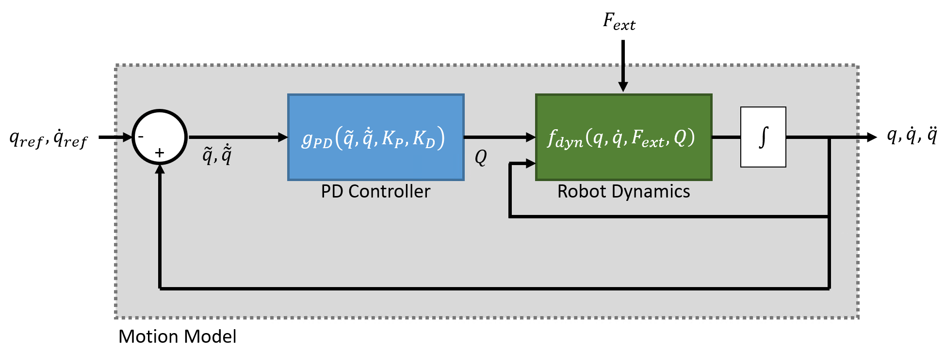
As with computed torque control, this system behavior uses the standard rigid-body robot dynamics, but uses the PD control law define the generalized force input :
where
— is the gravity torques and forces required for all joints to maintain their positions at the gravity specified in the Gravity property of the rigid body tree. Calculate the gravity torque by using the
gravityTorqueobject function.
The control input relies on these user-defined parameters:
— Proportional gain, specified as an -by- matrix, where is the number of movable joints of the manipulator
— Derivative gain, specified as an -by- matrix
Independent Joint Motion
When this system is modeled with independent joint motion, instead of modeling the closed loop system as standard rigid body robot dynamics plus a control input, each joint is instead modeled as a second-order system that already has the desired error behavior:
Inputs — This model accepts as the desired reference joint configuration and velocities, given as vectors. There is no external force input.
Outputs — The model outputs as the joint configuration, velocities, and accelerations. In the MATLAB version of the model, only accelerations are returned, and the user must choose an integrator or ODE solver to return the other states.
Complexity — This is low complexity. The motion model simply prescribes the error behavior that a position controller could aim to achieve.
When to apply — Use when the system has approximable error dynamics and there are no external force inputs required.
The system models the following closed-loop second order behavior for the *i-*th joint:
These parameters characterize the desired response defined for each joint:
— the natural frequency specified in units of
— t the damping ratio, which is unitless
Or as:
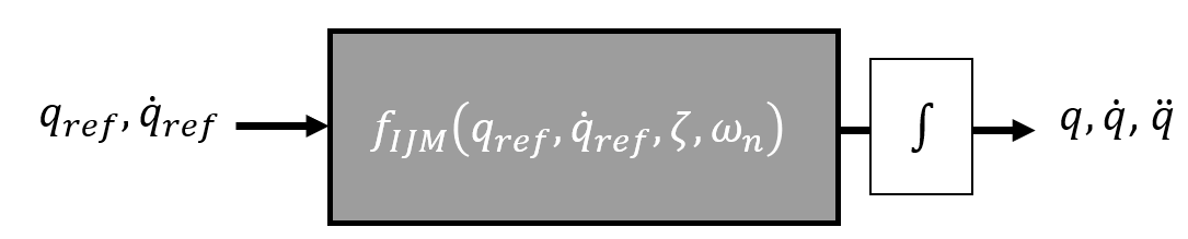
The complete system is therefore modeled as:
The model relies on these user-defined parameters:
— -by- diagonal matrix of natural frequencies in the NaturalFrequency property of the
jointSpaceMotionModelobject are in Hz ().— -by- diagonal matrix of the products of the squared natural frequencies , and damping ratios , specified in the DampingRatio property of the
jointSpaceMotionModelobject.
The values of and may be set directly, or they may be provided using the updateErrorDynamicsFromStep method, which computes values for and based on desired unit step response (defined using the transient behavior characteristics).
The Independent Joint Motion model represents a closed loop system under idealized behavior. In the absence of external forces and assuming no delays in the feedback (e.g. with continuous integration), the motion model using computed torque control produces an equivalent output.