bilin

Multivariable bilinear transform of frequency (s or z)

Syntax

GT = bilin(G,VERS,METHOD,AUG)

Description

bilin computes the effect on a system of the frequency-variable substitution,

$$s=\frac{\alpha z+\delta }{\gamma z+\beta }$$

The variable VERS denotes the transformation direction:

VERS= 1, forward transform (s→z) or $$(s\to \tilde{s})$$.

VERS=-1, reverse transform (z→s) or $$\left(\tilde{s}\to s\right)$$.

This transformation maps lines and circles to circles and lines in the complex plane. People often use this transformation to do sampled-data control system design [1] or, in general, to do shifting of jω modes [2], [3], [4].

Bilin computes several state-space bilinear transformations such as backward rectangular, etc., based on the METHOD you select

Bilinear Transform Types

Method	Type of bilinear transform
'BwdRec'	backward rectangular: $$s=\frac{z-1}{Tz}$$ AUG = T, the sample time.
'FwdRec'	forward rectangular: $$s=\frac{z-1}{T}$$ AUG = T, the sample time.
'S_Tust'	shifted Tustin: $$s=\frac{2}{T}\left(\frac{z-1}{\frac{z}{h}+1}\right)$$ AUG = [T h], is the “shift” coefficient.
'S_ftjw'	shifted jω-axis, bilinear pole-shifting, continuous-time to continuous-time: $$s=\frac{\tilde{s}+p_1}{1+\tilde{s}/p_2}$$ AUG = [p2 p1].
'G_Bili'	METHOD = 'G_Bili', general bilinear, continuous-time to continuous-time: $$s=\frac{\alpha \tilde{s}+\delta }{\gamma \tilde{s}+\beta }$$ AUG = $$\left[\alpha \beta \gamma \delta \right]$$.

Examples

Tustin Continuous s-Plane to Discrete z-Plane transforms

Consider the following continuous-time plant.

$$A=\left[\begin{array}{cc}-1& 1\\ 0& -2\end{array}\right],B=\left[\begin{array}{cc}1& 0\\ 1& 1\end{array}\right],C=\left[\begin{array}{cc}1& 0\\ 0& 1\end{array}\right],D=\left[\begin{array}{cc}0& 0\\ 0& 0\end{array}\right]$$.

A = [-1 1; 0 -2]; 
B = [1 0; 1 1];  
C = [1 0; 0 1];   
D = [0 0; 0 0]; 
sys = ss(A,B,C,D);                   

Discretize the plant at 20 Hz by several methods. Use c2d to compute the Tustin and pre-warped Tustin discretizations, and use bilin for the backward and forward rectangular discretizations.

Ts = 0.05;  % sample time
syst = c2d(sys,Ts,'tustin');         % Tustin 
sysp = c2d(sys,Ts,'prewarp',40);     % Pre-warped Tustin 
sysb = bilin(sys,1,'BwdRec',Ts);     % Backward Rectangular
sysf = bilin(sys,1,'FwdRec',Ts);     % Forward Rectangular

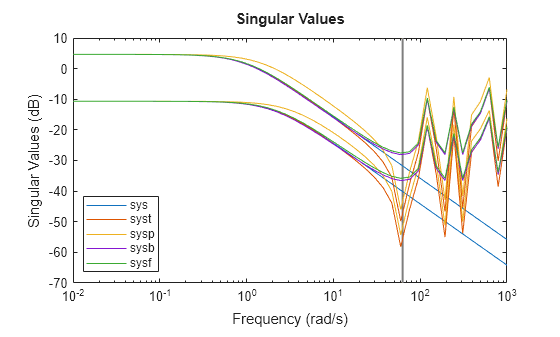
Plot the responses of the continuous-time plant and the transformed discrete-time plants.

w = logspace(-2,3,50); % frequencies to plot
sigma(sys,syst,sysp,sysb,sysf,w); 
legend('sys','syst','sysp','sysb','sysf','Location','SouthWest')

Bilinear continuous to continuous pole-shifting

Design an H mixed-sensitivity controller for a ACC Benchmark plant.

$$G(s)=\frac{1}{s^2(s^2+2)}$$

such that all closed-loop poles lie inside a circle in the left half of the s-plane whose diameter lies on between points [p1,p2]=[–12,–2]:

p1=-12; p2=-2; s=zpk('s');
G=ss(1/(s^2*(s^2+2)));          % original unshifted plant
Gt=bilin(G,1,'Sft_jw',[p1 p2]); % bilinear pole shifted plant Gt
Kt=mixsyn(Gt,1,[],1);           % bilinear pole shifted controller
K =bilin(Kt,-1,'Sft_jw',[p1 p2]); % final controller K

As shown in the following figure, closed-loop poles are placed in the left circle [p1 p2]. The shifted plant, which has its non-stable poles shifted to the inside the right circle, is

$$G_t(s)=4.765\times {10}^{-5}\frac{{(s-12)}^4}{{(s-2)}^2(s^2-4.274s+5.918)}$$

'S_ftjw' final closed-loop poles are inside the left [p1,p2] circle

Algorithms

bilin employs the state-space formulae in [3]:

$$\left[\begin{array}{cc}{A}_b& B_b\\ C_b& D_b\end{array}\right]=\left[\begin{array}{cc}(\beta A-\delta I){(\alpha I+\gamma A)}^{-1}& \left(\alpha \beta -\gamma \delta \right){\left(\alpha I-\gamma A\right)}^{-1}B\\ C{(\alpha I-\gamma A)}^{-1}& D+\gamma C{(\alpha I-\gamma A)}^{-1}B\end{array}\right]$$

References

[1] Franklin, G.F., and J.D. Powell, Digital Control of Dynamics System, Addison-Wesley, 1980.

[2] Safonov, M.G., R.Y. Chiang, and H. Flashner, “H_∞ Control Synthesis for a Large Space Structure,” AIAA J. Guidance, Control and Dynamics, 14, 3, p. 513-520, May/June 1991.

[3] Safonov, M.G., “Imaginary-Axis Zeros in Multivariable H_∞ Optimal Control”, in R.F. Curtain (editor), Modelling, Robustness and Sensitivity Reduction in Control Systems, p. 71-81, Springer-Varlet, Berlin, 1987.

[4] Chiang, R.Y., and M.G. Safonov, “H_∞ Synthesis using a Bilinear Pole Shifting Transform,” AIAA, J. Guidance, Control and Dynamics, vol. 15, no. 5, p. 1111-1117, September-October 1992.

Version History

Introduced before R2006a