orderwaveform
Extract time-domain order waveforms from vibration signal
Syntax
Description
xrec = orderwaveform(x,fs,rpm,orderList)x. x is
measured at a set rpm of rotational speeds expressed
in revolutions per minute. fs is the measurement
sample rate in Hz. The vector orderList specifies
the desired orders, whose waveforms are returned in the corresponding
columns of xrec. The function uses the Vold-Kalman
filter for the computation.
Examples
Create a simulated signal sampled at 600 Hz for 5 seconds. The system that is being tested increases its rotational speed from 10 to 40 revolutions per second (or, equivalently, from 600 to 2400 revolutions per minute) during the observation period.
Generate the tachometer readings.
fs = 600;
t1 = 5;
t = 0:1/fs:t1;

f0 = 10;
f1 = 40;
rpm = 60*linspace(f0,f1,length(t));
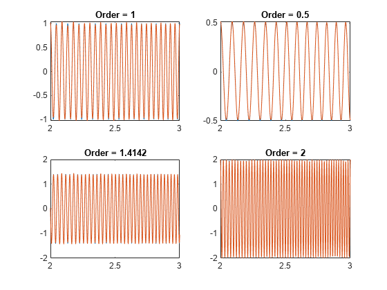
The signal consists of four harmonically related chirps with orders 1, 1/2, √2, and 2. The amplitudes of the chirps are 1, 1/2, √2, and 2, respectively. To generate the chirps, use the trapezoidal rule to express the phase as the integral of the rotational speed.
ord = [1 0.5 sqrt(2) 2];
amp = [1 0.5 sqrt(2) 2];

ph = 2*pi*cumtrapz(rpm/60)/fs;

x(1,:) = amp(1)*cos(ord(1)*ph);
x(2,:) = amp(2)*cos(ord(2)*ph);
x(3,:) = amp(3)*cos(ord(3)*ph);
x(4,:) = amp(4)*cos(ord(4)*ph);

xsum = sum(x);
Reconstruct the time-domain waveforms that compose the signal.
xrec = orderwaveform(xsum,fs,rpm,ord);
Visualize the results. Zoom in on a time interval occurring after the transients have decayed.
for kj = 1:4
    subplot(2,2,kj)
    plot(t,x(kj,:),t,xrec(:,kj))
    title("Order = " + ord(kj))
    xlim([2 3])
end
Create a simulated vibration signal consisting of two crossing orders corresponding to two different motors. The signal is sampled at 300 Hz for 3 seconds. The first motor increases its rotational speed from 10 to 100 revolutions per second (or, equivalently, from 600 to 6000 rpm) during the measurement. The second motor increases its rotational speed from 50 to 70 revolutions per second (or 3000 to 4200 rpm) during the same period.
fs = 300;
nsamp = 3*fs;

rpm1 = linspace(10,100,nsamp)'*60;
rpm2 = linspace(50,70,nsamp)'*60;
The measured signal is of order 1.2 and amplitude 2√2 with respect to the first motor. With respect to the second motor, the signal is of order 0.8 and amplitude 4√2.
x = [2 4]*sqrt(2).*cos(2*pi*cumtrapz([1.2*rpm1 0.8*rpm2]/60)/fs);
Make the first motor excite a resonance at the middle of the frequency range.
y = [1+1./(1+linspace(-10,10,nsamp).^4)'/2 ones(nsamp,1)].*x;

x = sum(y,2);
Visualize the orders using rpmfreqmap.
rpmfreqmap(x,fs,rpm1)

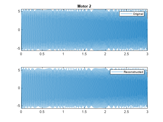
Reconstruct the time-domain waveforms that compose the signal. Use the Vold-Kalman algorithm to decouple the crossing orders.
xrec = orderwaveform(x,fs,[rpm1 rpm2],[1.2 0.8],[1 2],Decouple=true);
Plot the original and reconstructed waveforms.
for kj = 1:2
    figure(kj)
    subplot(2,1,1)
    plot((0:nsamp-1)/fs,y(:,kj))
    legend("Original")
    title("Motor" + kj)
    subplot(2,1,2)
    plot((0:nsamp-1)/fs,xrec(:,kj))
    legend("Reconstructed")
end
Input Arguments
Name-Value Arguments
Output Arguments
References
[1] Feldbauer, Christian, and Robert Höldrich. "Realization of a Vold-Kalman Tracking Filter — A Least Squares Problem." Proceedings of the COST G-6 Conference on Digital Audio Effects (DAFX-00). Verona, Italy, December 7–9, 2000.
[2] Vold, Håvard, and Jan Leuridan. "High Resolution Order Tracking at Extreme Slew Rates Using Kalman Tracking Filters." Shock and Vibration. Vol. 2, 1995, pp. 507–515.
Extended Capabilities
Version History
Introduced in R2016b
See Also
orderspectrum | ordertrack | rpmfreqmap | rpmordermap | tachorpm