Main Content

rpmordermap

Order-RPM map for order analysis

Description

map = rpmordermap(x,fs,rpm) returns the order-RPM map matrix, map, that results from performing order analysis on the input vector, x. x is measured at a set rpm of rotational speeds expressed in revolutions per minute. fs is the measurement sample rate in Hz. Each column of map contains root-mean-square (RMS) amplitude estimates of the orders present at each rpm value. rpmordermap resamples x to a constant samples-per-cycle rate and uses the short-time Fourier transform to analyze the spectral content of the resampled signal.

example

map = rpmordermap(x,fs,rpm,res) specifies the order resolution of the map in units of orders.

example

map = rpmordermap(___,Name,Value) specifies options using Name,Value pairs in addition to the input arguments in previous syntaxes.

example

[map,order,rpm,time,res] = rpmordermap(___) returns vectors with the orders, rotational speeds, and time instants at which the order map is computed. It also returns the order resolution used.

rpmordermap(___) with no output arguments plots the order map as a function of rotational speed and time on an interactive figure.

example

Examples

collapse all

Create a simulated signal sampled at 600 Hz for 5 seconds. The system that is being tested increases its rotational speed from 10 to 40 revolutions per second during the observation period.

Generate the tachometer readings.

fs = 600;
t1 = 5;
t = 0:1/fs:t1;

f0 = 10;
f1 = 40;
rpm = 60*linspace(f0,f1,length(t));

The signal consists of four harmonically related chirps with orders 1, 0.5, 4, and 6. The order-4 chirp has twice the amplitude of the others. To generate the chirps, use the trapezoidal rule to express the phase as the integral of the rotational speed.

o1 = 1;
o2 = 0.5;
o3 = 4;
o4 = 6;

ph = 2*pi*cumtrapz(rpm/60)/fs;

x = [1 1 2 1]*cos([o1 o2 o3 o4]'*ph);

Visualize the order-RPM map of the signal.

rpmordermap(x,fs,rpm)

Figure Order Map contains 5 axes objects and other objects of type uimenu, uitoolbar, uiflowcontainer. Hidden axes object 1 contains 2 objects of type line. Hidden axes object 2 contains 2 objects of type patch, text. Hidden axes object 3 contains 2 objects of type patch, text. Hidden axes object 4 contains 2 objects of type patch, text. Hidden axes object 5 contains 2 objects of type patch, text.

Analyze simulated data from an accelerometer placed in the cockpit of a helicopter.

Load the helicopter data. The vibrational measurements, vib, are sampled at a rate of 500 Hz for 10 seconds. Inspection of the data reveals that it has a linear trend. Remove the trend to prevent it from degrading the quality of the order estimation.

load('helidata.mat')

vib = detrend(vib);

Plot the nonlinear RPM profile. The rotor runs up until it reaches a maximum rotational speed of about 27,600 revolutions per minute and then coasts down.

plot(t,rpm)
xlabel('Time (s)')
ylabel('RPM')

Figure contains an axes object. The axes object with xlabel Time (s), ylabel RPM contains an object of type line.

Compute the order-RPM map. Specify an order resolution of 0.015.

[map,order,rpmOut,time] = rpmordermap(vib,fs,rpm,0.015);

Visualize the map.

imagesc(time,order,map)
ax = gca;
ax.YDir = 'normal';
xlabel('Time (s)')
ylabel('Order')

Figure contains an axes object. The axes object with xlabel Time (s), ylabel Order contains an object of type image.

Repeat the computation using a finer order resolution. Plot the map using the built-in functionality of rpmordermap. The lower orders are resolved more clearly.

rpmordermap(vib,fs,rpm,0.005)

Figure Order Map contains 5 axes objects and other objects of type uimenu, uitoolbar, uiflowcontainer. Hidden axes object 1 contains 2 objects of type line. Hidden axes object 2 contains 2 objects of type patch, text. Hidden axes object 3 contains 2 objects of type patch, text. Hidden axes object 4 contains 2 objects of type patch, text. Hidden axes object 5 contains 2 objects of type patch, text.

Generate a signal that consists of two linear chirps and a quadratic chirp, all sampled at 600 Hz for 5 seconds. The system that produces the signal increases its rotational speed from 10 to 40 revolutions per second during the testing period.

Generate the tachometer readings.

fs = 600;
t1 = 5;
t = 0:1/fs:t1;

f0 = 10;
f1 = 40;
rpm = 60*linspace(f0,f1,length(t));

The linear chirps have orders 1 and 2.5. The component with order 1 has twice the amplitude of the other. The quadratic chirp starts at order 6 and returns to this order at the end of the measurement. Its amplitude is 0.8. Create the signal using this information.

o1 = 1;
o2 = 2.5;
o6 = 6;

x = 2*chirp(t,o1*f0,t1,o1*f1)+chirp(t,o2*f0,t1,o2*f1) + ...
    0.8*chirp(t,o6*f0,t1,o6*f1,'quadratic');

Compute the order-RPM map of the signal. Use the peak amplitude at each measurement cell. Specify a resolution of 0.25 orders. Window the data with a Chebyshev window whose sidelobe attenuation is 80 dB.

[map,or,rp] = rpmordermap(x,fs,rpm,0.25, ...
    'Amplitude','peak','Window',{'chebwin',80});

Draw the order-RPM map as a waterfall plot.

[OR,RP] = meshgrid(or,rp);
waterfall(OR,RP,map')

view(-15,45)
xlabel('Order')
ylabel('RPM')
zlabel('Amplitude')

Figure contains an axes object. The axes object with xlabel Order, ylabel RPM contains an object of type patch.

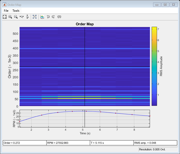
Plot an interactive order-RPM map by calling rpmordermap without output arguments.

Load the file helidata.mat, which contains simulated vibrational data from an accelerometer placed in the cockpit of a helicopter. The data is sampled at a rate of 500 Hz for 10 seconds. Remove the linear trend in the data. Call rpmordermap to generate an interactive plot of the order-RPM map. Specify an order resolution of 0.005 orders.

load helidata.mat
rpmordermap(detrend(vib),fs,rpm,0.005)

Figure Order Map contains 5 axes objects and other objects of type uimenu, uitoolbar, uiflowcontainer. Hidden axes object 1 contains 2 objects of type line. Hidden axes object 2 contains 2 objects of type patch, text. Hidden axes object 3 contains 2 objects of type patch, text. Hidden axes object 4 contains 2 objects of type patch, text. Hidden axes object 5 contains 2 objects of type patch, text.

See Algorithms for a more detailed description of the RPM-vs.-time plot at the bottom of the figure.

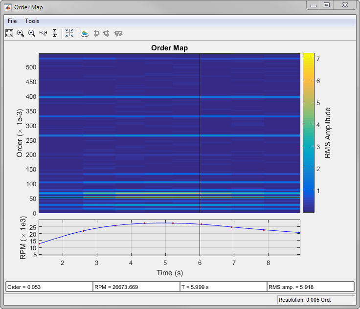
Move the crosshair cursors in the figure to determine the RPM and the RMS amplitude at order 0.053 after 6 seconds.

Figure Order Map contains 5 axes objects and other objects of type uimenu, uitoolbar, uiflowcontainer. Hidden axes object 1 contains 2 objects of type line. Hidden axes object 2 contains 2 objects of type patch, text. Hidden axes object 3 contains 2 objects of type patch, text. Hidden axes object 4 contains 2 objects of type patch, text. Hidden axes object 5 contains 2 objects of type patch, text.

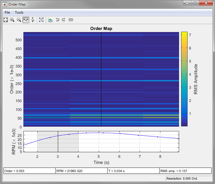
Click the Zoom X button in the toolbar to zoom into the time region between 2 and 4 seconds. The gray rectangle in the RPM-vs.-time plot shows the region of interest. You can slide this region to pan through time.

Figure Order Map contains 5 axes objects and other objects of type uimenu, uitoolbar, uiflowcontainer. Hidden axes object 1 contains 2 objects of type line. Hidden axes object 2 contains 2 objects of type patch, text. Hidden axes object 3 contains 2 objects of type patch, text. Hidden axes object 4 contains 2 objects of type patch, text. Hidden axes object 5 contains 2 objects of type patch, text.

Click the Waterfall Plot button to display the order-RPM map as a waterfall plot. For improved visibility, rotate the plot clockwise using the Rotate Left button three times. Move the panner to the interval between 5 and 7 seconds.

Figure Order Map contains 5 axes objects and other objects of type uimenu, uitoolbar, uiflowcontainer. Hidden axes object 1 contains 2 objects of type line. Hidden axes object 2 contains 2 objects of type patch, text. Hidden axes object 3 contains 2 objects of type patch, text. Hidden axes object 4 contains 2 objects of type patch, text. Hidden axes object 5 contains 2 objects of type patch, text.

Input Arguments

collapse all

Input signal, specified as a row or column vector.

Example: cos(pi/4*(0:159))+randn(1,160) specifies a sinusoid embedded in white Gaussian noise.

Sample rate, specified as a positive scalar expressed in Hz.

Rotational speeds, specified as a vector of positive values expressed in revolutions per minute. rpm must have the same length as x.

  • If you have a tachometer pulse signal, use tachorpm to extract rpm directly.

  • If you do not have a tachometer pulse signal, use rpmtrack to extract rpm from a vibration signal.

Example: 100:10:3000 specifies that a system rotates initially at 100 revolutions per minute and runs up to 3000 revolutions per minute in increments of 10.

Order resolution of the order-RPM map, specified as a positive scalar. If res is not specified, then rpmordermap sets it to the sample rate of the constant-samples-per-cycle signal divided by 256. If the resampled input signal is not long enough, then the function uses the entire resampled signal length to compute a single order estimate.

The actual order resolution may differ slightly from the specified value. For more details, see Algorithms.

Data Types: single | double

Name-Value Arguments

Specify optional pairs of arguments as Name1=Value1,...,NameN=ValueN, where Name is the argument name and Value is the corresponding value. Name-value arguments must appear after other arguments, but the order of the pairs does not matter.

Before R2021a, use commas to separate each name and value, and enclose Name in quotes.

Example: 'Scale','dB','Window','hann' specifies that the order map estimates are to be scaled in decibels and determined using a Hann window.

Order-RPM map amplitudes, specified as the comma-separated pair consisting of 'Amplitude' and one of 'rms', 'peak', or 'power'.

  • 'rms' — Returns the root-mean-square amplitude for each estimated order.

  • 'peak' — Returns the peak amplitude for each estimated order.

  • 'power' — Returns the power level for each estimated order.

Overlap percentage between adjoining segments, specified as the comma-separated pair consisting of 'OverlapPercent' and a scalar from 0 to 100. A value of 0 means that adjoining segments do not overlap. A value of 100 means that adjoining segments are shifted by one sample. A larger overlap percentage produces a smoother map but increases the computation time. See Algorithms for more information.

Data Types: double | single

Order-RPM map scaling, specified as the comma-separated pair consisting of 'Scale' and either 'linear' or 'dB'.

  • 'linear' — Returns a linearly scaled map.

  • 'dB' — Returns a logarithmic map with values expressed in decibels.

Analysis window, specified as the comma-separated pair consisting of 'Window' and one of these values:

  • 'flattopwin' specifies a flat top window. See flattopwin for more details.

  • 'chebwin' specifies a Chebyshev window. Use a cell array to specify a sidelobe attenuation in decibels. The sidelobe attenuation must be greater than 45 dB. If not specified, it defaults to 100 dB. See chebwin for more details.

  • 'hamming' specifies a Hamming window. See hamming for more details.

  • 'hann' specifies a Hann window. See hann for more details.

  • 'kaiser' specifies a Kaiser window. Use a cell array to specify a shape parameter, β. The shape parameter must be a positive scalar. If not specified, it defaults to 0.5. See kaiser for more details.

  • 'rectwin' specifies a rectangular window. See rectwin for more details.

Example: 'Window','chebwin' specifies a Chebyshev window with a sidelobe attenuation of 100 dB.

Example: 'Window',{'chebwin',60} specifies a Chebyshev window with a sidelobe attenuation of 60 dB.

Example: 'Window','kaiser' specifies a Kaiser window with a shape parameter of 0.5.

Example: 'Window',{'kaiser',1} specifies a Kaiser window with a shape parameter of 1.

Data Types: char | string | cell

Output Arguments

collapse all

Order-RPM map, returned as a matrix.

Orders, returned as a vector.

Rotational speeds, returned as a vector.

Time instants, returned as a vector.

Order resolution, returned as a scalar.

Algorithms

Order analysis is the study of vibrations in rotating systems that result from the rotation itself. The frequencies of these vibrations are often proportional to the rotational speed. The constants of proportionality are the orders.

The rotational speed is usually measured independently and changes with time under most experimental conditions. Proper analysis of rotation-induced vibrations requires resampling and interpolating the measured signal to achieve a constant number of samples per cycle. Through this process, the signal components whose frequencies are constant multiples of the rotational speed transform into constant tones. The transformation reduces the smearing of spectral components that occurs when frequency changes rapidly with time.

The rpmordermap function performs these steps:

  1. Uses cumtrapz to estimate the phase angle as the time integral of the rotational speed:

    ϕ(t)=0tRPM(τ)60dτ.

  2. Uses resample to upsample and lowpass-filter the signal. This step enables the function to interpolate the signal at nonsampled time points without aliasing of the high-frequency components. rpmordermap upsamples the signal by a factor of 15.

  3. Uses interp1 to interpolate the upsampled signal linearly onto a uniform grid in the phase domain. The highest accessible order in a measurement is fixed by the sample rate and the highest rotational speed reached by the system:

    Omax=fs/2max(RPM60).

    To capture this highest order accurately, it is necessary to sample the signal at twice Omax at least. For better results, rpmordermap oversamples by an extra factor of 4. The resulting phase-domain sample rate, fp, is

    fp=4×2Omax=4×2fs/2max(RPM60).

    By default, rpmordermap is configured to compute order-RPM matrices at a target order resolution

    r=fp256=4×602562×fs/2max(RPM)=1516fsmax(RPM),

    but you can specify a different value using the res input argument.

  4. Uses spectrogram to compute the short-time Fourier transform (STFT) of the interpolated signal. By default, the function divides the signal into L-sample segments and windows each of them with a flat top window. There are

    Noverlap=min(poverlap100×L,L1)

    samples of overlap between adjoining segments, where poverlap is specified using the 'OverlapPercent' name-value pair and defaults to 50%. The DFT length is set to L. The resolution is related to the sample rate and segment length through

    r=fpL×ENBW,

    where ENBW, the equivalent noise bandwidth of the window, is computed using enbw. Adjust the resolution to differentiate closely spaced orders. Smaller r values require larger segment lengths. ENBW itself depends on L, so L must be computed recursively for given r and fp. The resulting L value is usually not an integer, so rpmordermap rounds it using ceil. The actual order resolution may thus differ slightly from the specified target value. If you need to attain a given resolution, make sure that your signal has enough samples.

The red dots in the RPM-vs.-time plot at the bottom of the interactive rpmordermap window correspond to the right edge of each windowed segment. The blue line in the plot is the RPM signal drawn as a function of time:

Figure Order Map contains 5 axes objects and other objects of type uimenu, uitoolbar, uiflowcontainer. Hidden axes object 1 contains 2 objects of type line. Hidden axes object 2 contains 2 objects of type patch, text. Hidden axes object 3 contains 2 objects of type patch, text. Hidden axes object 4 contains 2 objects of type patch, text. Hidden axes object 5 contains 2 objects of type patch, text.

References

[1] Brandt, Anders. Noise and Vibration Analysis: Signal Analysis and Experimental Procedures. Chichester, UK: John Wiley & Sons, 2011.

Extended Capabilities

C/C++ Code Generation
Generate C and C++ code using MATLAB® Coder™.

Version History

Introduced in R2015b

expand all

Go to top of page