Main Content

Perform Hybrid Optimization Using sbiofit

This example shows how to configure sbiofit to perform a hybrid optimization by first running the global solver particleswarm, followed by another minimization function, fmincon.

Load Data

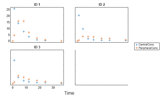
Load the sample data to fit. The data is stored as a table with variables ID, Time, CentralConc, and PeripheralConc. This synthetic data represents the time course of plasma concentrations measured at eight different time points for both central and peripheral compartments after an infusion dose for three individuals. The dose amount is 100 milligram and dose rate is 50 milligram/hour.

load('data10_32R.mat')
gData = groupedData(data);
gData.Properties.VariableUnits = {'','hour','milligram/liter','milligram/liter'};
sbiotrellis(gData,'ID','Time',{'CentralConc','PeripheralConc'},'Marker','+',...
            'LineStyle','none');

Figure contains 4 axes objects. Axes object 1 with title ID 1 contains 2 objects of type line. One or more of the lines displays its values using only markers Axes object 2 with title ID 2 contains 2 objects of type line. One or more of the lines displays its values using only markers Axes object 3 with title ID 3 contains 2 objects of type line. One or more of the lines displays its values using only markers These objects represent CentralConc, PeripheralConc. Axes object 4 is empty.

Create Model

Create a two-compartment model with an infusion dose.

pkmd                 = PKModelDesign;
pkc1                 = addCompartment(pkmd,'Central');
pkc1.DosingType      = 'Infusion';
pkc1.EliminationType = 'linear-clearance';
pkc1.HasResponseVariable = true;
pkc2                 = addCompartment(pkmd,'Peripheral');
model                = construct(pkmd);
configset            = getconfigset(model);
configset.CompileOptions.UnitConversion = true;
dose             = sbiodose('dose','TargetName','Drug_Central');
dose.StartTime   = 0;
dose.Amount      = 100;
dose.Rate        = 50;
dose.AmountUnits = 'milligram';
dose.TimeUnits   = 'hour';
dose.RateUnits   = 'milligram/hour';
responseMap = {'Drug_Central = CentralConc','Drug_Peripheral = PeripheralConc'};

Define Parameters to Estimate

Use the estimatedInfo object to define the estimated parameters.

paramsToEstimate   = {'log(Central)','log(Peripheral)','Q12','Cl_Central'};
estimatedParam     = estimatedInfo(paramsToEstimate,'InitialValue',[1 1 1 1],...
                                   'Bounds',[0 10]);

Define the Options for Hybrid Optimization

Define the options for the global solver and the hybrid solver. Because the parameters are bounded, make sure you use a compatible hybrid function for a constrained optimization, such as fmincon. Use optimset to define the options for fminsearch. Use optimoptions to define the options for fminunc, patternsearch, and fmincon.

rng('default');
globalMethod = 'particleswarm';
options = optimoptions(globalMethod);
hybridMethod = 'fmincon';
hybridopts = optimoptions(hybridMethod,'Display','none');
options = optimoptions(options,'HybridFcn',{hybridMethod,hybridopts});

Fit Data

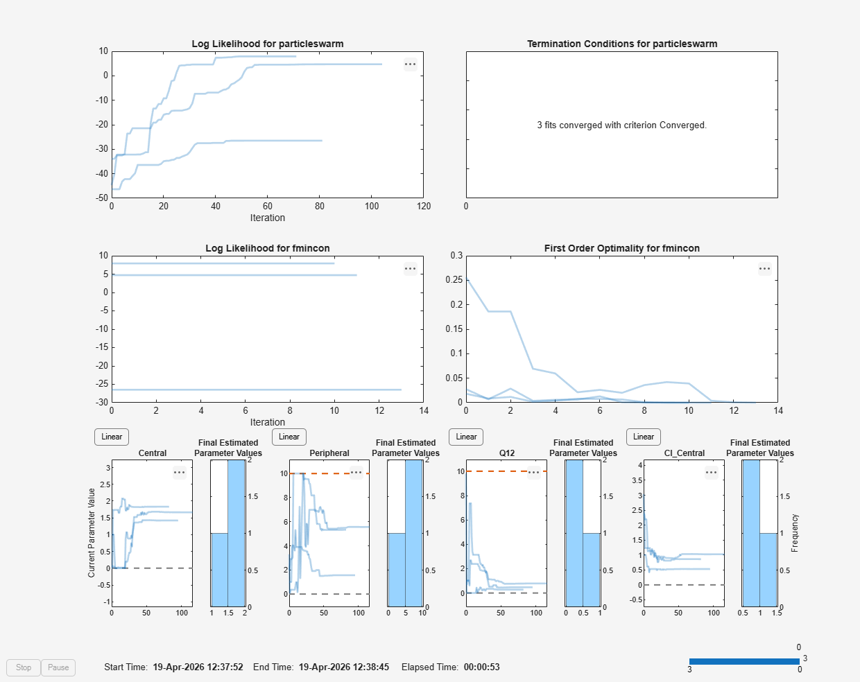
Estimate model parameters. Turn on ProgressPlot to see the live feedback on the status of fitting. The first row of plots are the quality measure plots for the global solver. The second row plots are for the hybrid function. For details, see Progress Plot.

unpooledFit =  sbiofit(model,gData,responseMap,estimatedParam,dose,globalMethod,...
                       options,'Pooled',false,'ProgressPlot',true);
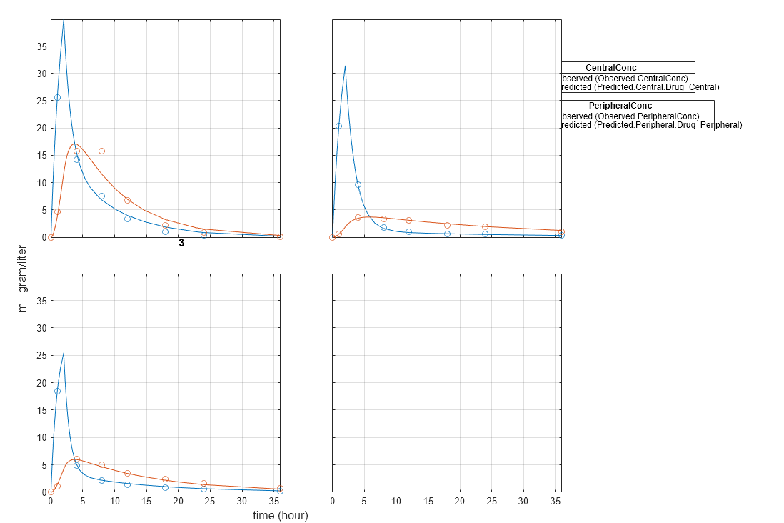
Figure Progress Plot for particleswarm with hybrid function fmincon contains 13 axes objects and other objects of type uicontrol, uipanel. Axes object 1 with title Log Likelihood for particleswarm, xlabel Iteration contains 3 objects of type line. Axes object 2 with title Termination Conditions for particleswarm contains an object of type text. These objects represent Failed, Converged. Axes object 3 with title Log Likelihood for fmincon, xlabel Iteration contains 3 objects of type line. Axes object 4 with title First Order Optimality for fmincon contains 3 objects of type line. Axes object 5 with title Central, ylabel Current Parameter Value contains 4 objects of type line. Axes object 6 with title Final Estimated Parameter Values contains an object of type histogram. Axes object 7 with title Peripheral contains 5 objects of type line. Axes object 8 with title Final Estimated Parameter Values contains an object of type histogram. Axes object 9 with title Q12 contains 5 objects of type line. Axes object 10 with title Final Estimated Parameter Values contains an object of type histogram. Axes object 11 with title Cl_Central contains 4 objects of type line. Axes object 12 with title Final Estimated Parameter Values, ylabel Frequency contains an object of type histogram. Hidden axes object 13 contains an object of type text.

Plot Results

plot(unpooledFit);

Figure contains 6 axes objects. Axes object 1 is empty. Axes object 2 with title 3 contains 4 objects of type line. One or more of the lines displays its values using only markers Axes object 3 with title 2 contains 4 objects of type line. One or more of the lines displays its values using only markers Axes object 4 with title 1 contains 4 objects of type line. One or more of the lines displays its values using only markers Hidden axes object 5 contains 2 objects of type line. One or more of the lines displays its values using only markers These objects represent Predicted (Predicted.Central.Drug_Central), Observed (Observed.CentralConc). Hidden axes object 6 contains 2 objects of type line. One or more of the lines displays its values using only markers These objects represent Predicted (Predicted.Peripheral.Drug_Peripheral), Observed (Observed.PeripheralConc).

See Also

Related Topics