Estimate Constrained Values of a Lookup Table

Objectives

This example shows how to estimate constrained values of a lookup table in the Parameter Estimator. Apply monotonically increasing constraints to the lookup table output values, and use the Parameter Estimator to estimate the table values.

About the Data

In this example, use lookup_increasing.mat, which contains the measured I/O data for estimating the lookup table values. The MAT-file includes the following variables:

xdata1 — Input data consisting of 602 uniformly sampled data points in the range [-5,5].
ydata1 — Output data corresponding to the input data samples.
time1 — Time vector.

Use the I/O data to estimate monotonically increasing output values of the lookup table in the lookup_increasing Simulink^® model.

Lookup Table Increasing Constraints Models

Open Live Script

Open the lookup table model.

open_system('lookup_increasing.slx')

This command opens the Simulink® model, and loads the estimation data in the MATLAB® workspace.

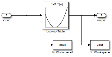
Lookup Table Output

View the table output values by double-clicking the Lookup Table block.

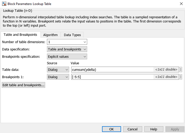
The table contains 11 output values at breakpoints [-5:5], specified in the Function Block Parameters dialog box. To learn more about how to specify the table values, see Enter Breakpoints and Table Data.

The Table data field shows that the table output values are the cumulative sum of the values stored in variable ydelta. Thus, if y_n are the 11 table output values, ydelta is (y₁, y₂–y₁, y₃–y₂, ..., y₁₁–y₁₀). The initial ydelta values are loaded from lookup_increasing.mat.

The initial table output values are not monotonically increasing. To ensure monotonically increasing table output values, the difference between adjacent table output values should be positive. To do so, estimate ydelta in the Parameter Estimator using the measured I/O estimation data, and constrain ydelta(2:end) to be positive during estimation.

Estimate the Monotonically Increasing Table Values Using Default Settings

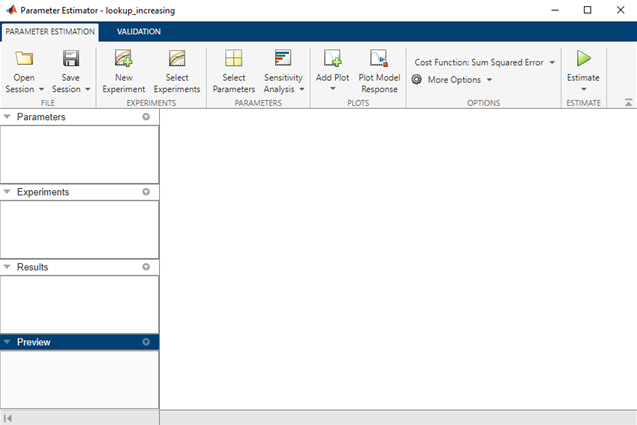
Open a parameter estimation session.
In the Simulink model, select Parameter Estimator from the Apps tab, in the gallery, under Control Systems to open a session with the name lookup_increasing in the Parameter Estimator.
Create an experiment and import the I/O data.
On the Parameter Estimation tab, click New Experiment. Type [time1,ydata1] in Outputs and [time1,xdata1] in Inputs of the Edit Experiment dialog box. Click OK. A new experiment with name Exp is created in the Experiments area of the app. Rename the experiment EstimationData by right-clicking the default experiment name, Exp, and selecting Rename. For more information, see Import Data for Parameter Estimation.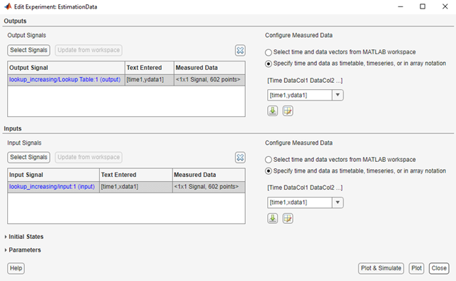

Run an initial simulation to view the measured data, simulated model values, and the initial table values by typing the following commands at the MATLAB^® prompt.

sim('lookup_increasing')
figure(1)
plot(xdata1,ydata1,'m*',xout,yout,'b^')
hold on
plot(-5:5,cumsum(ydelta),'k','LineWidth',2)
xlabel('Input Data')
ylabel('Output Data')
legend('Measured data',...
    'Initial simulated data',...
    'Initial table output')

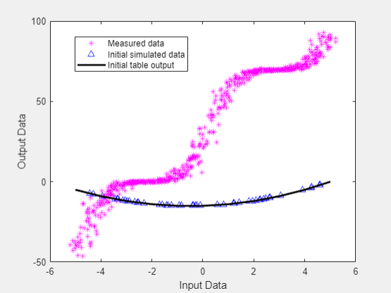
The initial table output values and simulated data do not match the measured data.

Select parameter for estimation.
On the Parameter Estimation tab, click Select Parameters. The Edit: Estimated Parameters dialog box opens. In the Parameters Tuned for all Experiments panel, click Select parameters to open the Select Model Variables dialog box. Check the box next to ydelta, and click OK.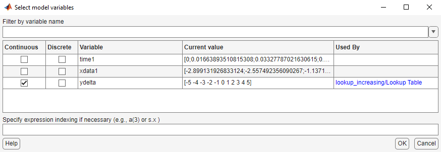
The ydelta values are selected for estimation by default in the Edit: Estimated Parameters dialog box.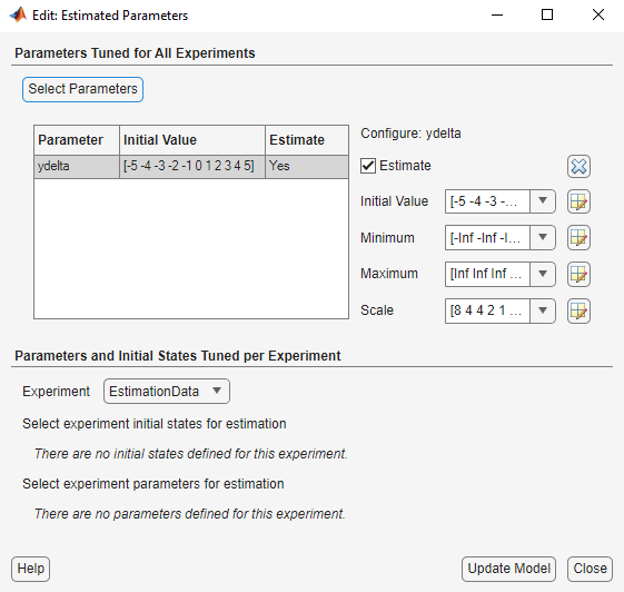
Apply a monotonically increasing constraint on the table output values. For more details about the table, see Lookup Table Output.
In the Edit: Estimated Parameters dialog box, click the arrow next to the ydelta values. In the expanded menu, set Minimum ydelta values to [-Inf,zeros(1,10)]. Thus, while the first value in ydelta can by anything, subsequent values which are the difference between adjacent table output values, must be positive.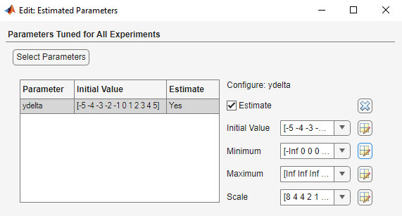
Select EstimationData experiment for estimation.
On the Parameter Estimation tab, click Select Experiment. By default, EstimationData is selected for estimation. If not, check the box under the Estimation column, and click OK.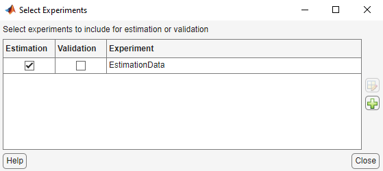
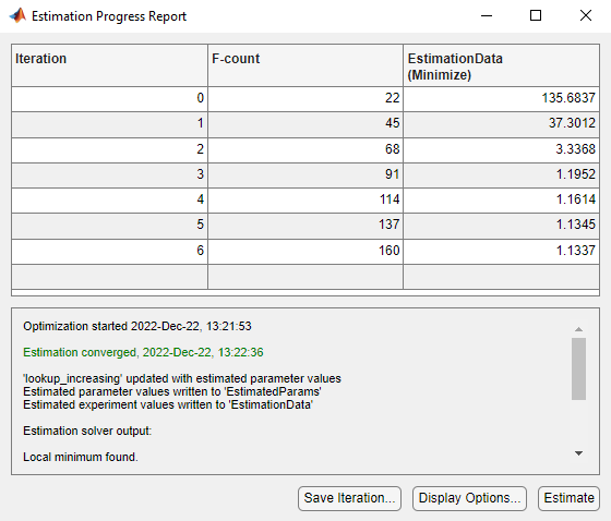
Estimate the table values using default settings.
On the Parameter Estimation tab, click Estimate.
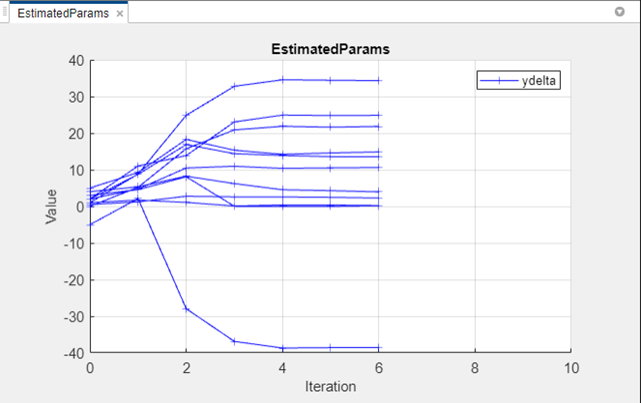
The Parameter Trajectory plot shows the change in the parameter values at each iteration.
The Estimation Progress Report shows the iteration number, number of times the objective function is evaluated, and value of the cost function at the end of each iteration.
The estimated parameters are saved in a new variable, EstimatedParams, in the Results area of the app. To view the estimated parameters, right-click EstimatedParams and select Open.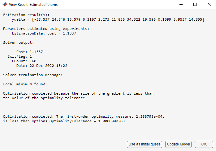
The estimated ydelta(2:end) values are positive. Thus, the output of the table, which is the cumulative sum of the values stored in ydelta, is monotonically increasing.

Validate the Estimation Results

After you estimate the table values, as described in Estimate the Monotonically Increasing Table Values Using Default Settings, you use another measured data set to validate and check that you have not over-fit the model. You can plot and examine the following plots to validate the estimation results:

Residuals plot
Measured and simulated data plots

Create an experiment to use for validation and import the validation I/O data.
On the Parameter Estimation tab, click New Experiment. Type [time2,ydata2] in Outputs and [time2,xdata2] in Inputs of the Edit Experiment dialog box. Name the experiment ValidationData by right-clicking the default experiment name, Exp, in the Experiments area of the app, and selecting Rename. For more information, see Import Data for Parameter Estimation.
Select the experiment for validation.
Click Select Experiments on the Parameter Estimation tab. The ValidationData experiment is selected for estimation by default. Clear Estimation and select the box for Validation.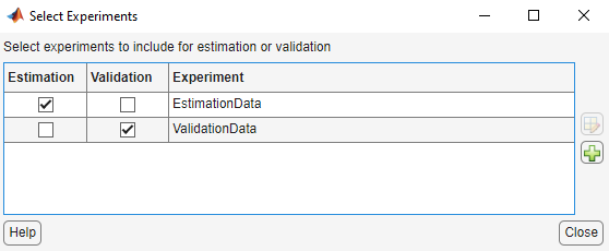
Select the results to validate.
On the Validation tab, click Select Results to Validate. Clear Use current parameter values, select EstimatedParams, and click OK.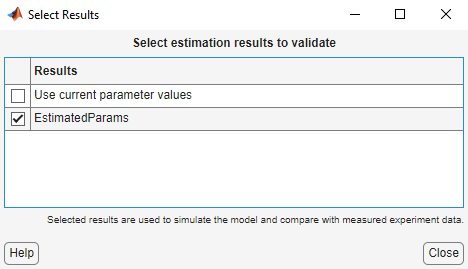
Select the plots to display during validation.
The Parameter Estimator displays the experiment plot after validation by default. Add the residuals plot by selecting the corresponding box on the Validation tab.

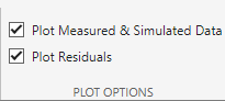
Click Validate.
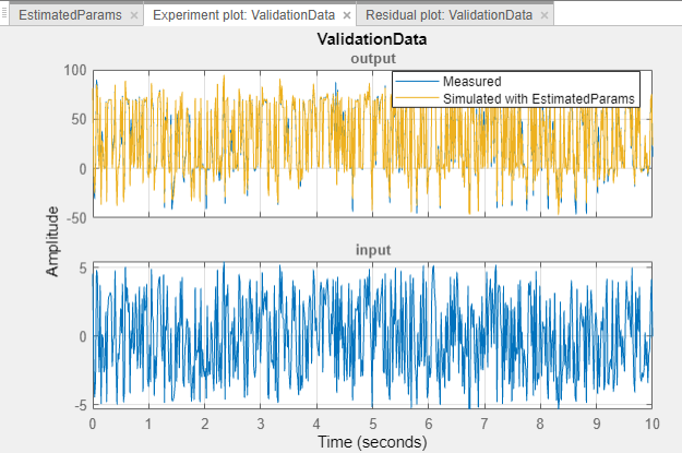
Examine the plots.
1. The experiment plot shows the data simulated using estimated parameters agrees with the measured validation data.
2. To view the residuals plot, click Residual plot: ValidationData tab.
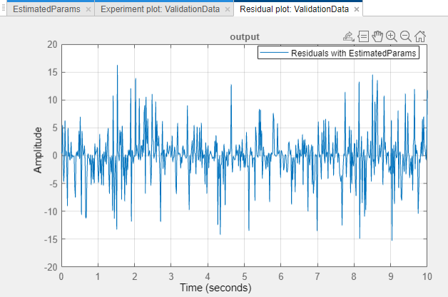
  The residuals, which show the difference between the simulated and measured data, lie within 15% of the maximum output variation. This indicates a good match between the measured and simulated table data values.
3. Plot and examine the validation data, simulated data, and estimated table values.
  sim('lookup_increasing') figure(2); plot(xdata2,ydata2,'m*',xout,yout,'b^') hold on; plot(-5:5,cumsum(ydelta),'k','LineWidth', 2) xlabel('Input Data'); ylabel('Output Data'); legend('Validation data','Simulated data','Table output values');
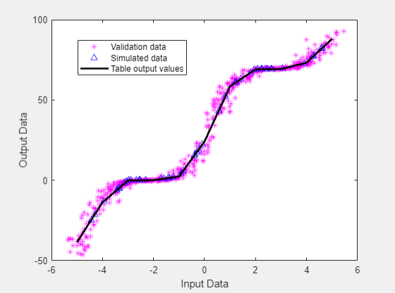
  The table output values match both the measured data and the simulated table values. The table output values cover the entire range of input values, which indicates that all the lookup table values have been estimated.