Simulink Subsystems as States

By using a Simulink^® subsystem within a Stateflow^® state, you can model hybrid dynamic systems or systems that switch between periodic and continuous time dynamics. In your Stateflow chart, you can use Simulink based states to model a periodic or continuous dynamic system combined with switching logic that uses transitions. You can access inputs and outputs from your chart within each Simulink based state. Simulink based states are not supported in standalone Stateflow charts in MATLAB^®.

To initialize Simulink blocks when switching between Simulink based states, use Stateflow textual notation or Simulink State Reader and State Writer blocks.

To create linked Simulink based states, use libraries to save action subsystems. When you copy an action subsystem from a library model into a Stateflow chart, it appears as a linked Simulink based state. When you update the library block, the changes are reflected in all Stateflow charts containing the block.

Using Simulink based states means that you do not have to use complex textual syntax in Stateflow to model hybrid systems.

When to Use Simulink Based States

Use Simulink based states when:

You want to model hybrid dynamic systems that include continuous or periodic dynamics.
The structure of the system dynamics change substantially between the various modes of operation, for example, modeling PID controllers.

For systems where you call logic intermittently, use Simulink functions.

When the structure of the Simulink algorithm remains substantially unchanged, but certain gains or parameters switch between various models, use Simulink logic outside of Stateflow. An example of this type of algorithm is gain scheduling. See Model Gain-Scheduled Control Systems in Simulink (Simulink Control Design).

Model a Pole Vaulter by Using Simulink Based States

This example uses:

Open Model

This Stateflow chart models a person moving through the stages of pole vaulting by using Simulink based states.

The first stage is the approach run of the vaulter, which is modeled in the Simulink based state Run_up. In the second stage, the vaulter plants the pole and takes off, which is modeled by the Simulink based state Take_off. The final stage happens when the vaulter clears the bar and releases the pole, which is modeled by the Simulink based state Fly.

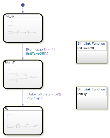
The states Run_up and Fly are easier to model by using Cartesian coordinates. The state Take_off is easier to model by using polar coordinates. To switch from one coordinate system to another, use Simulink functions InitTakeOff and InitFly.

Model the Approach of the Pole Vaulter

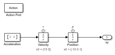
The default state in the chart PoleVaulter is Run_up. This state models the pole vaulter traveling along the ground toward the jump. The pole vaulter starts at -10 on the $x$ -axis and runs toward zero. As the pole vaulter moves along the ground, the position of the pole vaulter in the xy-plane is continuously changing, but the state of running remains the same. In this model, the integrator blocks Position and Velocity are state owner blocks for State Reader blocks in the Simulink function InitTakeOff. This subsystem outputs the Cartesian coordinates of the pole vaulter.

Convert Cartesian Coordinates to Polar Coordinates

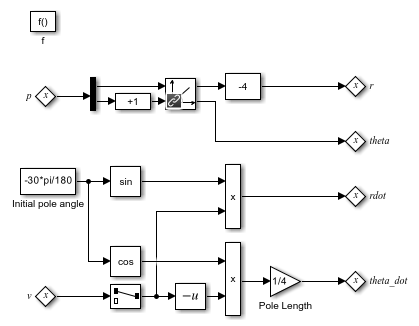
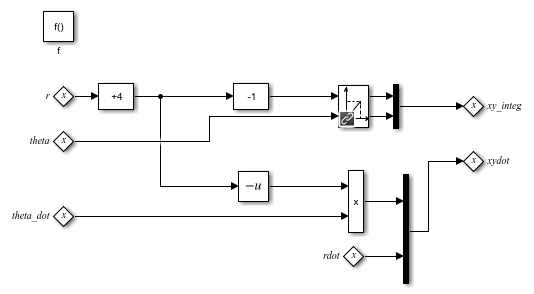
The transition from Run_up to Take_off occurs when the position of the pole vaulter along the $x$ -axis, Run_up.p(1), becomes greater than -4. During the transition InitTakeOff is initialized, the State Reader block connects to its owner block, and the function is executed. This function converts the Cartesian coordinates from Position and Velocity to polar coordinates, r, theta, rdot, and theta_dot. These coordinates are output as State Writer blocks, which are connected to owner blocks in the state Take_off. The Simulink function InitTakeOff contains this logic:

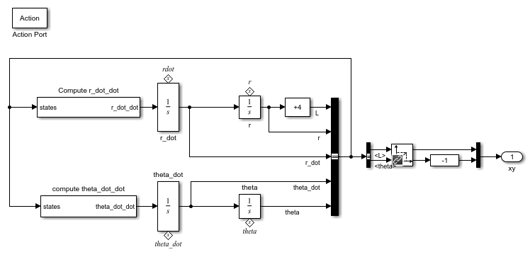
Model the Take Off of the Pole Vaulter

When the position of the pole vaulter along the $x$ -axis, Run_up.p(1), becomes greater than -4, the Simulink based state Take_off becomes the active state. This state models the pole vaulter during the take off phase of the jump. This subsystem outputs the Cartesian coordinates of the pole vaulter.

Convert Polar Coordinates to Cartesian Coordinates

The transition from Take_off to Fly occurs when the angle of the pole vaulter, theta, becomes less than $\pi/2$ . During the transition, InitFly is initialized, the State Reader block connects to its owner block, and the function is executed. This function converts the polar coordinates r, theta, rdot, and theta_dot to Cartesian coordinates, xy_integ and xydot. These coordinates are output as State Writer blocks, which are connected to owner blocks in the state Fly. The Simulink function InitFly contains this logic:

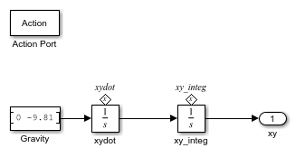
Model the Free Fall of the Pole Vaulter

When the angle of the pole vaulter, theta, is less than $\pi/2$ , the Simulink based state Fly becomes the active state. This state models the pole vaulter after the jump has cleared and the pole vaulter is falling to the ground. As the pole vaulter falls, the position of the pole vaulter in the x-y plane is continuously changing, but the state of falling remains the same. In this model, the integrator blocks xydot and xy_integ are state owner blocks for State Writer blocks in the Simulink function InitFly. This subsystem outputs the Cartesian coordinates of the pole vaulter.

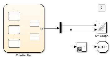
The Record block shows the results of this simulation.

Limitations

You cannot use Simulink based states with:

Moore charts
Discrete Event charts
HDL Coder
PLC Coder
Simulink Code Inspector
Super step transitions

Simulink based states do not support debugging.