Main Content

loss

Loss of ECOC incremental learning classification model on batch of data

Since R2022a

    Description

    loss returns the classification loss of a configured multiclass error-correcting output codes (ECOC) classification model for incremental learning (incrementalClassificationECOC object).

    To measure model performance on a data stream and store the results in the output model, call updateMetrics or updateMetricsAndFit.

    example

    L = loss(Mdl,X,Y) returns the classification error of the ECOC classification model for incremental learning Mdl using the batch of predictor data X and corresponding responses Y.

    example

    L = loss(Mdl,X,Y,Name=Value) uses additional options specified by one or more name-value arguments. For example, you can specify a decoding scheme and classification loss function.

    Examples

    collapse all

    The performance of an incremental model on streaming data is measured in three ways:

    • Cumulative metrics measure the performance since the start of incremental learning.

    • Window metrics measure the performance on a specified window of observations. The metrics are updated every time the model processes the specified window.

    • The loss function measures the performance on a specified batch of data only.

    Load the human activity data set. Randomly shuffle the data.

    load humanactivity
    n = numel(actid);
    rng(1) % For reproducibility
    idx = randsample(n,n);
    X = feat(idx,:);
    Y = actid(idx);

    For details on the data set, enter Description at the command line.

    Create an ECOC classification model for incremental learning. Specify the class names and a metrics window size of 1000 observations. Configure the model for loss by fitting it to the first 10 observations.

    Mdl = incrementalClassificationECOC(ClassNames=unique(Y),MetricsWindowSize=1000);
    initobs = 10;
    Mdl = fit(Mdl,X(1:initobs,:),Y(1:initobs));

    Mdl is an incrementalClassificationECOC model. All its properties are read-only.

    Simulate a data stream, and perform the following actions on each incoming chunk of 100 observations:

    1. Call updateMetrics to measure the cumulative performance and the performance within a window of observations. Overwrite the previous incremental model with a new one to track performance metrics.

    2. Call loss to measure the model performance on the incoming chunk.

    3. Call fit to fit the model to the incoming chunk. Overwrite the previous incremental model with a new one fitted to the incoming observations.

    4. Store all performance metrics to see how they evolve during incremental learning.

    % Preallocation
    numObsPerChunk = 100;
    nchunk = floor((n - initobs)/numObsPerChunk);
    mc = array2table(zeros(nchunk,3),VariableNames=["Cumulative","Window","Chunk"]);
    
    % Incremental learning
    for j = 1:nchunk
        ibegin = min(n,numObsPerChunk*(j-1) + 1 + initobs);
        iend   = min(n,numObsPerChunk*j + initobs);
        idx = ibegin:iend;    
        Mdl = updateMetrics(Mdl,X(idx,:),Y(idx));
        mc{j,["Cumulative","Window"]} = Mdl.Metrics{"ClassificationError",:};
        mc{j,"Chunk"} = loss(Mdl,X(idx,:),Y(idx));
        Mdl = fit(Mdl,X(idx,:),Y(idx));
    end

    Mdl is an incrementalClassificationECOC model object trained on all the data in the stream. During incremental learning and after the model is warmed up, updateMetrics checks the performance of the model on the incoming observations, and then the fit function fits the model to those observations. loss is agnostic of the metrics warm-up period, so it measures the classification error for every chunk.

    To see how the performance metrics evolve during training, plot them.

    plot(mc.Variables)
    xlim([0 nchunk])
    ylabel("Classification Error")
    xline(Mdl.MetricsWarmupPeriod/numObsPerChunk,"--")
    grid on
    legend(mc.Properties.VariableNames)
    xlabel("Iteration")

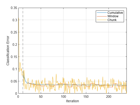
    The yellow line represents the classification error on each incoming chunk of data. After the metrics warm-up period, Mdl tracks the cumulative and window metrics.

    Fit an ECOC classification model for incremental learning to streaming data, and compute the minimum average binary loss on the incoming chunks of data.

    Load the human activity data set. Randomly shuffle the data.

    load humanactivity
    n = numel(actid);
    rng(1) % For reproducibility
    idx = randsample(n,n);
    X = feat(idx,:);
    Y = actid(idx);

    For details on the data set, enter Description at the command line.

    Create an ECOC classification model for incremental learning. Configure the model as follows:

    • Specify the class names.

    • Specify a metrics warm-up period of 1000 observations.

    • Specify a metrics window size of 2000 observations.

    • Track the minimal average binary loss to measure the performance of the model. Create an anonymous function that measures the minimal average binary loss of each new observation. Create a structure array containing the name MinimalLoss and its corresponding function handle.

    • Compute the classification loss by fitting the model to the first 10 observations.

    tolerance = 1e-10;
    minimalBinaryLoss = @(~,S,~)min(-S,[],2);
    ce = struct("MinimalLoss",minimalBinaryLoss);
    
    Mdl = incrementalClassificationECOC(ClassNames=unique(Y), ...
        MetricsWarmupPeriod=1000,MetricsWindowSize=2000, ...
        Metrics=ce);
    initobs = 10;
    Mdl = fit(Mdl,X(1:initobs,:),Y(1:initobs));

    Mdl is an incrementalClassificationECOC model object configured for incremental learning.

    Perform incremental learning. At each iteration:

    • Simulate a data stream by processing a chunk of 100 observations.

    • Call updateMetrics to compute cumulative and window metrics on the incoming chunk of data. Overwrite the previous incremental model with a new one fitted to overwrite the previous metrics.

    • Call loss to compute the minimum average binary loss on the incoming chunk of data. Whereas the cumulative and window metrics require that custom losses return the loss for each observation, loss requires the loss for the entire chunk. Compute the mean of the losses within a chunk.

    • Call fit to fit the incremental model to the incoming chunk of data.

    • Store the cumulative, window, and chunk metrics to see how they evolve during incremental learning.

    % Preallocation
    numObsPerChunk = 100;
    nchunk = floor((n - initobs)/numObsPerChunk);
    tanloss = array2table(zeros(nchunk,3), ...
        VariableNames=["Cumulative","Window","Chunk"]);
    
    % Incremental fitting
    for j = 1:nchunk
        ibegin = min(n,numObsPerChunk*(j-1) + 1 + initobs);
        iend   = min(n,numObsPerChunk*j + initobs);
        idx = ibegin:iend;    
        Mdl = updateMetrics(Mdl,X(idx,:),Y(idx));
        tanloss{j,1:2} = Mdl.Metrics{"MinimalLoss",:};
        tanloss{j,3} = loss(Mdl,X(idx,:),Y(idx), ...
            LossFun=@(z,zfit,w)mean(minimalBinaryLoss(z,zfit,w)));
        Mdl = fit(Mdl,X(idx,:),Y(idx));
    end

    Mdl is an incrementalClassificationECOC model object trained on all the data in the stream. During incremental learning and after the model is warmed up, updateMetrics checks the performance of the model on the incoming observations, and then the fit function fits the model to those observations.

    Plot the performance metrics to see how they evolve during incremental learning.

    semilogy(tanloss.Variables)
    xlim([0 nchunk])
    ylabel("Minimal Average Binary Loss")
    xline(Mdl.MetricsWarmupPeriod/numObsPerChunk,"-.")
    xlabel("Iteration")
    legend(tanloss.Properties.VariableNames)

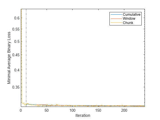
    The plot suggests the following:

    • updateMetrics computes the performance metrics after the metrics warm-up period only.

    • updateMetrics computes the cumulative metrics during each iteration.

    • updateMetrics computes the window metrics after processing 2000 observations (20 iterations).

    • Because Mdl is configured to predict observations from the beginning of incremental learning, loss can compute the minimum average binary loss on each incoming chunk of data.

    Input Arguments

    collapse all

    ECOC classification model for incremental learning, specified as an incrementalClassificationECOC model object. You can create Mdl by calling incrementalClassificationECOC directly, or by converting a supported, traditionally trained machine learning model using the incrementalLearner function.

    You must configure Mdl to predict labels for a batch of observations.

    • If Mdl is a converted, traditionally trained model, you can predict labels without any modifications.

    • Otherwise, you must fit Mdl to data using fit or updateMetricsAndFit.

    Batch of predictor data, specified as a floating-point matrix of n observations and Mdl.NumPredictors predictor variables. The value of the ObservationsIn name-value argument determines the orientation of the variables and observations. The default ObservationsIn value is "rows", which indicates that observations in the predictor data are oriented along the rows of X.

    The length of the observation labels Y and the number of observations in X must be equal; Y(j) is the label of observation j (row or column) in X.

    Note

    loss supports only floating-point input predictor data. If your input data includes categorical data, you must prepare an encoded version of the categorical data. Use dummyvar to convert each categorical variable to a numeric matrix of dummy variables. Then, concatenate all dummy variable matrices and any other numeric predictors. For more details, see Dummy Variables.

    Data Types: single | double

    Batch of labels, specified as a categorical, character, or string array, a logical or floating-point vector, or a cell array of character vectors.

    The length of the observation labels Y and the number of observations in X must be equal; Y(j) is the label of observation j (row or column) in X.

    If Y contains a label that is not a member of Mdl.ClassNames, the loss function issues an error. The data type of Y and Mdl.ClassNames must be the same.

    Data Types: char | string | cell | categorical | logical | single | double

    Name-Value Arguments

    Specify optional pairs of arguments as Name1=Value1,...,NameN=ValueN, where Name is the argument name and Value is the corresponding value. Name-value arguments must appear after other arguments, but the order of the pairs does not matter.

    Example: BinaryLoss="quadratic",Decoding="lossbased" specifies the quadratic binary learner loss function and the loss-based decoding scheme for aggregating the binary losses.

    Binary learner loss function, specified as a built-in loss function name or function handle.

    • This table describes the built-in functions, where yj is the class label for a particular binary learner (in the set {–1,1,0}), sj is the score for observation j, and g(yj,sj) is the binary loss formula.

      ValueDescriptionScore Domaing(yj,sj)
      "binodeviance"Binomial deviance(–∞,∞)log[1 + exp(–2yjsj)]/[2log(2)]
      "exponential"Exponential(–∞,∞)exp(–yjsj)/2
      "hamming"Hamming[0,1] or (–∞,∞)[1 – sign(yjsj)]/2
      "hinge"Hinge(–∞,∞)max(0,1 – yjsj)/2
      "linear"Linear(–∞,∞)(1 – yjsj)/2
      "logit"Logistic(–∞,∞)log[1 + exp(–yjsj)]/[2log(2)]
      "quadratic"Quadratic[0,1][1 – yj(2sj – 1)]2/2

      The software normalizes binary losses so that the loss is 0.5 when yj = 0. Also, the software calculates the mean binary loss for each class [1].

    • For a custom binary loss function, for example customFunction, specify its function handle BinaryLoss=@customFunction.

      customFunction has this form:

      bLoss = customFunction(M,s)

      • M is the K-by-B coding matrix stored in Mdl.CodingMatrix.

      • s is the 1-by-B row vector of classification scores.

      • bLoss is the classification loss. This scalar aggregates the binary losses for every learner in a particular class. For example, you can use the mean binary loss to aggregate the loss over the learners for each class.

      • K is the number of classes.

      • B is the number of binary learners.

      For an example of a custom binary loss function, see Predict Test-Sample Labels of ECOC Model Using Custom Binary Loss Function. This example is for a traditionally trained model. You can define a custom loss function for incremental learning as shown in the example.

    For more information, see Binary Loss.

    Data Types: char | string | function_handle

    Decoding scheme, specified as "lossweighted" or "lossbased".

    The decoding scheme of an ECOC model specifies how the software aggregates the binary losses and determines the predicted class for each observation. The software supports two decoding schemes:

    • "lossweighted" — The predicted class of an observation corresponds to the class that produces the minimum sum of the binary losses over binary learners.

    • "lossbased" — The predicted class of an observation corresponds to the class that produces the minimum average of the binary losses over binary learners.

    For more information, see Binary Loss.

    Example: Decoding="lossbased"

    Data Types: char | string

    Loss function, specified as "classiferror" (classification error) or a function handle for a custom loss function.

    To specify a custom loss function, use function handle notation. The function must have this form:

    lossval = lossfcn(C,S,W)

    • The output argument lossval is an n-by-1 floating-point vector, where n is the number of observations in X. The value in lossval(j) is the classification loss of observation j.

    • You specify the function name (lossfcn).

    • C is an n-by-K logical matrix with rows indicating the class to which the corresponding observation belongs. K is the number of distinct classes (numel(Mdl.ClassNames), and the column order corresponds to the class order in the ClassNames property. Create C by setting C(p,q) = 1, if observation p is in class q, for each observation in the specified data. Set the other element in row p to 0.

    • S is an n-by-K numeric matrix of predicted classification scores. S is similar to the NegLoss output of predict, where rows correspond to observations in the data and the column order corresponds to the class order in the ClassNames property. S(p,q) is the classification score of observation p being classified in class q.

    • W is an n-by-1 numeric vector of observation weights.

    Example: LossFun=@lossfcn

    Data Types: char | string | function_handle

    Predictor data observation dimension, specified as "rows" or "columns".

    Example: ObservationsIn="columns"

    Data Types: char | string

    Batch of observation weights, specified as a floating-point vector of positive values. loss weighs the observations in the input data with the corresponding values in Weights. The size of Weights must equal n, which is the number of observations in the input data.

    By default, Weights is ones(n,1).

    For more details, see Observation Weights.

    Example: Weights=W specifies the observation weights as the vector W.

    Data Types: double | single

    Output Arguments

    collapse all

    Classification loss, returned as a numeric scalar. L is a measure of model quality. Its interpretation depends on the loss function and weighting scheme.

    More About

    collapse all

    Classification Error

    The classification error has the form

    L=j=1nwjej,

    where:

    • wj is the weight for observation j. The software renormalizes the weights to sum to 1.

    • ej = 1 if the predicted class of observation j differs from its true class, and 0 otherwise.

    In other words, the classification error is the proportion of observations misclassified by the classifier.

    Binary Loss

    The binary loss is a function of the class and classification score that determines how well a binary learner classifies an observation into the class. The decoding scheme of an ECOC model specifies how the software aggregates the binary losses and determines the predicted class for each observation.

    Assume the following:

    • mkj is element (k,j) of the coding design matrix M—that is, the code corresponding to class k of binary learner j. M is a K-by-B matrix, where K is the number of classes, and B is the number of binary learners.

    • sj is the score of binary learner j for an observation.

    • g is the binary loss function.

    • k^ is the predicted class for the observation.

    The software supports two decoding schemes:

    • Loss-based decoding [2] (Decoding is 'lossbased') — The predicted class of an observation corresponds to the class that produces the minimum average of the binary losses over all binary learners.

      k^=argmink1Bj=1B|mkj|g(mkj,sj).

    • Loss-weighted decoding [3] (Decoding is 'lossweighted') — The predicted class of an observation corresponds to the class that produces the minimum average of the binary losses over the binary learners for the corresponding class.

      k^=argminkj=1B|mkj|g(mkj,sj)j=1B|mkj|.

      The denominator corresponds to the number of binary learners for class k. [1] suggests that loss-weighted decoding improves classification accuracy by keeping loss values for all classes in the same dynamic range.

    The predict, resubPredict, and kfoldPredict functions return the negated value of the objective function of argmin as the second output argument (NegLoss) for each observation and class.

    This table summarizes the supported binary loss functions, where yj is a class label for a particular binary learner (in the set {–1,1,0}), sj is the score for observation j, and g(yj,sj) is the binary loss function.

    ValueDescriptionScore Domaing(yj,sj)
    "binodeviance"Binomial deviance(–∞,∞)log[1 + exp(–2yjsj)]/[2log(2)]
    "exponential"Exponential(–∞,∞)exp(–yjsj)/2
    "hamming"Hamming[0,1] or (–∞,∞)[1 – sign(yjsj)]/2
    "hinge"Hinge(–∞,∞)max(0,1 – yjsj)/2
    "linear"Linear(–∞,∞)(1 – yjsj)/2
    "logit"Logistic(–∞,∞)log[1 + exp(–yjsj)]/[2log(2)]
    "quadratic"Quadratic[0,1][1 – yj(2sj – 1)]2/2

    The software normalizes binary losses so that the loss is 0.5 when yj = 0, and aggregates using the average of the binary learners [1].

    Do not confuse the binary loss with the overall classification loss (specified by the LossFun name-value argument of the loss and predict object functions), which measures how well an ECOC classifier performs as a whole.

    Algorithms

    collapse all

    Observation Weights

    If the prior class probability distribution is known (in other words, the prior distribution is not empirical), loss normalizes observation weights to sum to the prior class probabilities in the respective classes. This action implies that the default observation weights are the respective prior class probabilities.

    If the prior class probability distribution is empirical, the software normalizes the specified observation weights to sum to 1 each time you call loss.

    References

    [1] Allwein, E., R. Schapire, and Y. Singer. “Reducing multiclass to binary: A unifying approach for margin classifiers.” Journal of Machine Learning Research. Vol. 1, 2000, pp. 113–141.

    [2] Escalera, S., O. Pujol, and P. Radeva. “Separability of ternary codes for sparse designs of error-correcting output codes.” Pattern Recog. Lett. Vol. 30, Issue 3, 2009, pp. 285–297.

    [3] Escalera, S., O. Pujol, and P. Radeva. “On the decoding process in ternary error-correcting output codes.” IEEE Transactions on Pattern Analysis and Machine Intelligence. Vol. 32, Issue 7, 2010, pp. 120–134.

    Version History

    Introduced in R2022a