Nonparametric Estimates of Cumulative Distribution Functions and Their Inverses
This example shows how to estimate the cumulative distribution function (CDF) from data in a nonparametric or semiparametric way. It also illustrates the inversion method for generating random numbers from the estimated CDF. The Statistics and Machine Learning Toolbox™ includes more than two dozen random number generator functions for parametric univariate probability distributions. These functions allow you to generate random inputs for a wide variety of simulations, however, there are situations where it is necessary to generate random values to simulate data that are not described by a simple parametric family.
The toolbox also includes the functions pearsrnd and johnsrnd, for generating random values without having to specify a parametric distribution from which to draw--those functions allow you to specify a distribution in terms of its moments or quantiles, respectively.
However, there are still situations where even more flexibility is needed, to generate random values that "imitate" data that you have collected even more closely. In this case, you might use a nonparametric estimate of the CDF of those data, and use the inversion method to generate random values. The inversion method involves generating uniform random values on the unit interval, and transforming them to a desired distribution using the inverse CDF for that distribution.
From the opposite perspective, it is sometimes desirable to use a nonparametric estimate of the CDF to transform observed data onto the unit interval, giving them an approximate uniform distribution.
The ecdf function computes one type of nonparametric CDF estimate, the empirical CDF, which is a stairstep function. This example illustrates some smoother alternatives, which may be more suitable for simulating or transforming data from a continuous distribution.
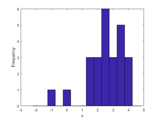
For the purpose of illustration, here are some simple simulated data. There are only 25 observations, a small number chosen to make the plots in the example easier to read. The data are also sorted to simplify plotting.
rng(19,'twister');
n = 25;
x = evrnd(3,1,n,1); x = sort(x);
hist(x,-2:.5:4.5);
xlabel('x'); ylabel('Frequency');
A Piecewise Linear Nonparametric CDF Estimate
The ecdf function provides a simple way to compute and plot a "stairstep" empirical CDF for data. In the simplest cases, this estimate makes discrete jumps of 1/n at each data point.
[Fi,xi] = ecdf(x);
stairs(xi,Fi,'r');
xlim([-2.5 5]); xlabel('x'); ylabel('F(x)');

This estimate is useful for many purposes, including investigating the goodness of fit of a parametric model to data. Its discreteness, however, may make it unsuitable for use in empirically transforming continuous data to or from the unit interval.
It is simple to modify the empirical CDF to address that problem. Instead of taking discrete jumps of 1/n at each data point, define a function that is piecewise linear, with breakpoints at the midpoints of those jumps. The height at each of the data points is then [1/2n, 3/2n, ..., (n-1/2)/n], instead of [(1/n), (2/n), ..., 1]. Use the output of ecdf to compute those breakpoints, and then "connect the dots" to define the piecewise linear function.
xj = xi(2:end);
Fj = (Fi(1:end-1)+Fi(2:end))/2;
hold on
plot(xj,Fj,'b.', xj,Fj,'b-');
hold off
legend({'ECDF' 'Breakpoints' 'Piecewise Linear Estimate'},'location','NW');

Because ecdf deals appropriately with repeated values and censoring, this calculation works even in cases with more complicated data than in this example.
Since the smallest data point corresponds to a height of 1/2n, and the largest to 1-1/2n, the first and last linear segments must be extended beyond the data, to make the function reach 0 and 1.
xj = [xj(1)-Fj(1)*(xj(2)-xj(1))/((Fj(2)-Fj(1)));
      xj;
      xj(n)+(1-Fj(n))*((xj(n)-xj(n-1))/(Fj(n)-Fj(n-1)))];
Fj = [0; Fj; 1];
hold on
plot(xj,Fj,'b-','HandleVisibility','off');
hold off
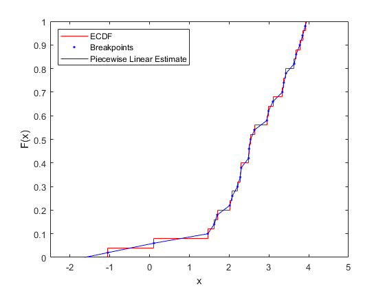
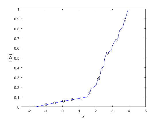
This piecewise linear function provides a nonparametric estimate of the CDF that is continuous and symmetric. Evaluating it at points other than the original data is just a matter of linear interpolation, and it can be convenient to define an anonymous function to do that.
F = @(y) interp1(xj,Fj,y,'linear','extrap');
y = linspace(-1,3.75,10);
plot(xj,Fj,'b-',y,F(y),'ko');
xlim([-2.5 5]); xlabel('x'); ylabel('F(x)');
A Piecewise Linear Nonparametric Inverse CDF Estimate
You can use the same calculations to compute a nonparametric estimate of the inverse CDF. In fact, the inverse CDF estimate is just the CDF estimate with the axes swapped.
stairs(Fi,[xi(2:end); xi(end)],'r');
hold on
plot(Fj,xj,'b-');
hold off
ylim([-2.5 5]); ylabel('x'); xlabel('F(x)');
legend({'ECDF' 'Piecewise Linear Estimate'},'location','NW');
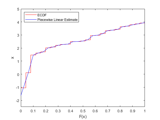
Evaluating this nonparametric inverse CDF at points other than the original breakpoints is again just a matter of linear interpolation. For example, generate uniform random values and use the CDF estimate to transform them back to the scale of your original observed data. This is the inversion method.
Finv = @(u) interp1(Fj,xj,u,'linear','extrap');
u = rand(10000,1);
hist(Finv(u),-2:.25:4.5);
xlabel('x'); ylabel('Frequency');
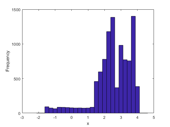
Notice that this histogram of simulated data is more spread out than the histogram of the original data. This is due, in part, to the much larger sample size--the original data consist of only 25 values. But it is also because the piecewise linear CDF estimate, in effect, "spreads out" each of the original observations over an interval, and more so in regions where the individual observations are well-separated.
For example, the two individual observations to the left of zero correspond to a wide, flat region of low density in the simulated data. In contrast, in regions where the data are closely spaced, towards the right tail, for example, the piecewise linear CDF estimate "spreads out" the observations to a lesser extent. In that sense, the method performs a simple version of what is known as variable bandwidth smoothing. However, despite the smoothing, the simulated data retain most of the idiosyncrasies of the original data, i.e., the regions of high and low density.
Kernel Estimators for the CDF and Inverse CDF
Instead of estimating the CDF using a piecewise linear function, you can perform kernel estimation using the ksdensity function to make a smooth nonparametric estimate. Though it is often used to make a nonparametric density estimate, ksdensity can also estimate other functions. For example, to transform your original data to the unit interval, use it to estimate the CDF.
F = ksdensity(x, x, 'function','cdf', 'width',.35);
stairs(xi,Fi,'r');
hold on
plot(x,F,'b.');
hold off
xlim([-2.5 5]); xlabel('x'); ylabel('F(x)');
legend({'ECDF' 'Kernel Estimates'},'location','NW');

ksdensity also provides a convenient way to evaluate the kernel CDF estimate at points other than the original data. For example, plot the estimate as a smooth curve.
y = linspace(-2.5,5,1000);
Fy = ksdensity(x, y, 'function','cdf', 'width',.35);
stairs(xi,Fi,'r');
hold on
plot(y,Fy,'b-');
hold off
legend({'ECDF' 'Kernel Estimate'},'location','NW');
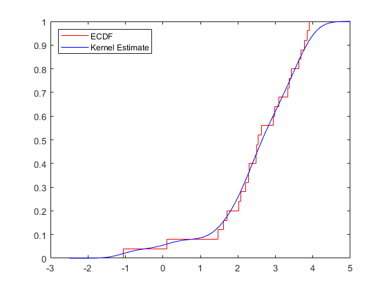
ksdensity uses a bandwidth parameter to control the amount of smoothing in the estimates it computes, and it is possible to let ksdensity choose a default value. The examples here use a fairly small bandwidth to limit the amount of smoothing. Even so, the kernel estimate does not follow the ECDF as closely as the piecewise linear estimate does.
One way to estimate the inverse CDF using kernel estimation is to compute the kernel CDF estimate on a grid of points spanning the range of the original data, and then use the same procedure as for the piecewise linear estimate. For example, to plot the inverse CDF kernel estimate as a smooth curve, simply swap the axes.
stairs(Fi,[xi(2:end); xi(end)],'r');
hold on
plot(Fy,y,'b-');
hold off
ylim([-2.5 5]); ylabel('x'); xlabel('F(x)');
legend({'ECDF' 'Kernel Estimate'},'location','NW');
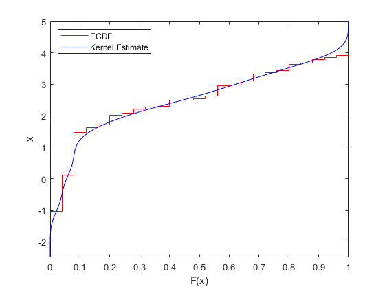
To transform uniform random values back to the scale of the original data, interpolate using the grid of CDF estimates.
Finv = @(u) interp1(Fy,y,u,'linear','extrap');
hist(Finv(u),-2.5:.25:5);
xlabel('x'); ylabel('Frequency');

Notice that the simulated data using the kernel CDF estimate has not completely "smoothed over" the two individual observations to the left of zero present in the original data. The kernel estimate uses a fixed bandwidth. With the particular bandwidth value used in this example, those two observations contribute to two localized areas of density, rather than a wide flat region as was the case with the piecewise linear estimate. In contrast, the kernel estimate has smoothed the data more in the right tail than the piecewise linear estimate.
Another way to generate simulated data using kernel estimation is to use ksdensity to compute an estimate of the inverse CDF directly, again using the 'function' parameter. For example, transform those same uniform values.
r = ksdensity(x, u, 'function','icdf', 'width',.35);
However, using the latter method can be time-consuming for large amounts of data. A simpler, but equivalent, method is to resample with replacement from the original data and add some appropriate random noise.
r = datasample(x,100000,'replace',true) + normrnd(0,.35,100000,1);
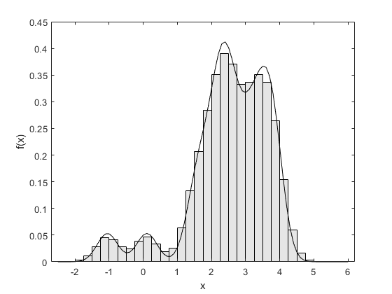
If you generate enough random values, a histogram of the result follows the kernel density estimate of the original data very closely.
binwidth = .25;
edges = -2.5:binwidth:6;
ctrs = edges(1:end-1) + binwidth./2;
counts = histc(r,edges); counts = counts(1:end-1);
bar(ctrs,counts./(sum(counts).*binwidth),1,'FaceColor',[.9 .9 .9]);
hold on
xgrid = edges(1):.1:edges(end);
fgrid = ksdensity(x, xgrid, 'function','pdf', 'width',.3);
plot(xgrid,fgrid,'k-');
hold off
xlabel('x'); ylabel('f(x)');
A Semiparametric CDF Estimate
A nonparametric CDF estimate requires a good deal of data to achieve reasonable precision. In addition, data only affect the estimate "locally." That is, in regions where there is a high density of data, the estimate is based on more observations than in regions where there is a low density of data. In particular, nonparametric estimates do not perform well in the tails of a distribution, where data are sparse by definition.
Fitting a semiparametric model to your data using the paretotails function allows the best of both the nonparametric and parametric worlds. In the "center" of the distribution, the model uses the piecewise linear nonparametric estimate for the CDF. In each tail, it uses a generalized Pareto distribution. The generalized Pareto is often used as a model for the tail(s) of a dataset, and while it is flexible enough to fit a wide variety of distribution tails, it is sufficiently constrained so that it requires few data to provide a plausible and smooth fit to tail data.
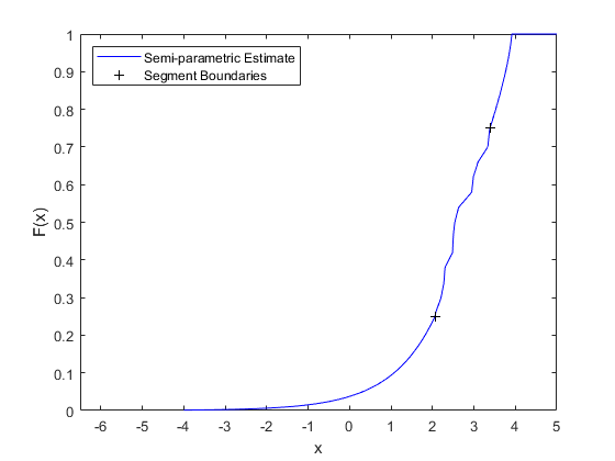
For example, you might define the "center" of the data as the middle 50%, and specify that the transitions between the nonparametric estimate and the Pareto fits take place at the .25 and .75 quantiles of your data. To evaluate the CDF of the semiparametric model fit, use the fit's cdf method.
semipFit = paretotails(x,.25,.75);
Warning: Problem fitting generalized Pareto distribution to upper tail. Maximum
likelihood has converged to a boundary point of the parameter space.
The warning is due to using so few data -- 6 points in each tail in this case -- and indicates that the fitted generalized Pareto distribution in the upper tail extends exactly to the smallest observation, and no further. You can see that in the histogram shown below. In a real application, you would usually have more data, and the warning would typically not occur.
[p,q] = boundary(semipFit);
y = linspace(-4,6,1000);
Fy = cdf(semipFit,y);
plot(y,Fy,'b-', q,p,'k+');
xlim([-6.5 5]); xlabel('x'); ylabel('F(x)');
legend({'Semi-parametric Estimate' 'Segment Boundaries'},'location','NW');
To transform uniform random values back to the scale of your original data, use the fit's icdf method.
r = icdf(semipFit,u);
hist(r,-6.5:.25:5);
xlabel('x'); ylabel('Frequency');

This semiparametric estimate has smoothed the tails of the data more than the center, because of the parametric model used in the tails. In that sense, the estimate is more similar to the piecewise linear estimate than to the kernel estimate. However, it is also possible to use paretotails to create a semiparametric fit that uses kernel estimation in the center of the data.
Conclusions
This example illustrates three methods for computing a nonparametric or semiparametric CDF or inverse CDF estimate from data. The three methods impose different amounts and types of smoothing on the data. Which method you choose depends on how each method captures or fails to capture what you consider the important features of your data.