RegressionQuantileLinear

Quantile linear regression model

Since R2024b

Description

A RegressionQuantileLinear object is a trained quantile linear regression model. For each quantile (Quantiles), the object stores the estimated linear model coefficients (Beta) and estimated bias term (Bias). The object also contains the regularization strength used for all quantiles (Lambda).

After training a RegressionQuantileLinear model object, you can use the loss object function to compute the quantile loss, and the predict object function to predict the response for new data.

Creation

Create a RegressionQuantileLinear object by using the fitrqlinear function.

Properties

Linear Regression Properties

Quantiles — Quantiles

Read-only: vector of values in the range [0,1]

This property is read-only.

Quantiles used to train the quantile linear regression model, returned as a vector of values in the range [0,1].

Data Types: double

Beta — Linear coefficient estimates

Read-only: numeric matrix

This property is read-only.

Linear coefficient estimates, returned as a numeric matrix. Each row corresponds to an expanded predictor (ExpandedPredictorNames), and each column corresponds to a quantile (Quantiles).

Data Types: double

Bias — Estimated bias terms

Read-only: numeric vector

This property is read-only.

Estimated bias terms or model intercepts, returned as a numeric vector. Each element corresponds to a quantile (Quantiles).

Data Types: double

Lambda — Regularization term strength

Read-only: nonnegative scalar

This property is read-only.

Regularization term strength for the ridge (L2) penalty, returned as a nonnegative scalar. The software uses the same regularization term strength for all quantiles.

Data Types: double | single

Solver — Objective function minimization technique

Read-only: 'bfgs' | 'lbfgs'

This property is read-only.

Objective function minimization technique used to train the quantile linear regression model, returned as 'bfgs' or 'lbfgs'.

Data Types: char

ModelParameters — Parameter values used to train model

Read-only: QuantileLinearParams object

This property is read-only.

Parameter values used to train the quantile linear regression model, returned as a QuantileLinearParams object. ModelParameters contains parameter values such as the name-value arguments used to train the model.

Access the properties of ModelParameters by using dot notation. For example, you can access the initial linear coefficient estimates used to train a model Mdl by using Mdl.ModelParameters.Beta.

ConvergenceInfo — Convergence information

Read-only: structure array

This property is read-only.

Convergence information, returned as a structure array.

Field	Description
Lambda	Regularization term strength
Objective	Objective function value for each quantile when the training optimization ends
IterationLimit	Maximum number of training optimization iterations
NumIterations	Number of iterations used to train the model for each quantile
GradientNorm	Gradient magnitude at the last iteration for each quantile
GradientTolerance	Absolute gradient tolerance
RelativeChangeInBeta	Relative change in the linear coefficients at the last iteration for each quantile
BetaTolerance	Relative tolerance on the linear coefficients and the bias term
TerminationCode	Code for TerminationStatus
TerminationStatus	Criterion for ending the training optimization
History	Training history
FitTime	Total time spent fitting the model for each quantile (in seconds)

Data Types: struct

Predictor Properties

PredictorNames — Predictor variable names

Read-only: cell array of character vectors

This property is read-only.

Predictor variable names, returned as a cell array of character vectors. The order of the elements of PredictorNames corresponds to the order in which the predictor names appear in the training data.

Data Types: cell

CategoricalPredictors — Categorical predictor indices

Read-only: vector of positive integers | []

This property is read-only.

Categorical predictor indices, returned as a vector of positive integers. Assuming that the predictor data contains observations in rows, CategoricalPredictors contains index values corresponding to the columns of the predictor data that contain categorical predictors. If none of the predictors are categorical, then this property is empty ([]).

Data Types: double

ExpandedPredictorNames — Expanded predictor names

Read-only: cell array of character vectors

This property is read-only.

Expanded predictor names, returned as a cell array of character vectors. If the model uses encoding for categorical variables, then ExpandedPredictorNames includes the names that describe the expanded variables. Otherwise, ExpandedPredictorNames is the same as PredictorNames.

Data Types: cell

Mu — Predictor means

Read-only: numeric vector | []

This property is read-only.

Predictor means, returned as a numeric vector. If you set Standardize to 1 or true when you train the linear model, then the length of the Mu vector is equal to the number of expanded predictors (ExpandedPredictorNames). The vector contains 0 values for dummy variables corresponding to expanded categorical predictors.

If you set Standardize to 0 or false when you train the linear model, then the Mu value is an empty vector ([]).

Data Types: double

Sigma — Predictor standard deviations

Read-only: numeric vector | []

This property is read-only.

Predictor standard deviations, returned as a numeric vector. If you set Standardize to 1 or true when you train the linear model, then the length of the Sigma vector is equal to the number of expanded predictors (ExpandedPredictorNames). The vector contains 1 values for dummy variables corresponding to expanded categorical predictors.

If you set Standardize to 0 or false when you train the linear model, then the Sigma value is an empty vector ([]).

Data Types: double

X — Unstandardized predictors

Read-only: numeric matrix | table

This property is read-only.

Unstandardized predictors used to train the linear model, returned as a numeric matrix or table. X retains its original orientation, with observations in rows or columns depending on the value of the ObservationsIn name-value argument in the call to fitrqlinear.

Data Types: single | double | table

Response Properties

ResponseName — Response variable name

Read-only: character vector

This property is read-only.

Response variable name, returned as a character vector.

Data Types: char

Y — Response values

Read-only: numeric vector

This property is read-only.

Response values used to train the model, returned as a numeric vector. Each row of Y represents the response value of the corresponding observation in X.

Data Types: single | double

ResponseTransform — Response transformation function

"none" | function handle

Response transformation function, specified as "none" or a function handle. ResponseTransform describes how the software transforms raw response values.

For a MATLAB^® function or a function that you define, enter its function handle. For example, you can enter Mdl.ResponseTransform = @function, where function accepts a numeric vector of the original responses and returns a numeric vector of the same size containing the transformed responses.

Data Types: char | string | function_handle

Other Data Properties

HyperparameterOptimizationResults — Cross-validation optimization of hyperparameters

Read-only: BayesianOptimization object | table | []

Since R2025a

This property is read-only.

Cross-validation optimization of hyperparameters, returned as a BayesianOptimization object or a table of hyperparameters and associated values. This property is nonempty if the OptimizeHyperparameters name-value argument is nonempty when you create the model. The value of HyperparameterOptimizationResults depends on the setting of the Optimizer option in the HyperparameterOptimizationOptions value when you create the model.

Value of Optimizer Option	Value of HyperparameterOptimizationResults
"bayesopt" (default)	Object of class BayesianOptimization
"gridsearch" or "randomsearch"	Table of hyperparameters used, observed objective function values (cross-validation loss), and rank of observations from lowest (best) to highest (worst)

NumObservations — Number of observations

Read-only: positive numeric scalar

This property is read-only.

Number of observations in the training data stored in X and Y, returned as a positive numeric scalar.

Data Types: double

RowsUsed — Observations of original training data stored

Read-only: logical vector | []

This property is read-only.

Observations of the original training data stored in the model, returned as a logical vector. This property is empty if all observations are stored in X and Y.

Data Types: logical

W — Observation weights

Read-only: numeric vector

This property is read-only.

Observation weights used to train the model, returned as an n-by-1 numeric vector. n is the number of observations (NumObservations).

The software normalizes the observation weights specified by the Weights name-value argument in the call to fitrqlinear so that the elements of W sum to 1.

Data Types: single | double

Object Functions

compact	Reduce size of machine learning model
crossval	Cross-validate machine learning model
loss	Loss for quantile linear regression model
predict	Predict response for quantile linear regression model

Examples

Fit Quantile Linear Regression Model

Fit a quantile linear regression model using the 0.25, 0.50, and 0.75 quantiles.

Load the carbig data set, which contains measurements of cars made in the 1970s and early 1980s. Create a matrix X containing the predictor variables Acceleration, Displacement, Horsepower, and Weight. Store the response variable MPG in the variable Y.

load carbig
X = [Acceleration,Displacement,Horsepower,Weight];
Y = MPG;

Delete rows of X and Y where either array has missing values.

R = rmmissing([X Y]);
X = R(:,1:end-1);
Y = R(:,end);

Partition the data into training data (XTrain and YTrain) and test data (XTest and YTest). Reserve approximately 20% of the observations for testing, and use the rest of the observations for training.

rng(0,"twister") % For reproducibility of the partition
c = cvpartition(length(Y),"Holdout",0.20);

trainingIdx = training(c);
XTrain = X(trainingIdx,:);
YTrain = Y(trainingIdx);

testIdx = test(c);
XTest = X(testIdx,:);
YTest = Y(testIdx);

Train a quantile linear regression model. Specify to use the 0.25, 0.50, and 0.75 quantiles (that is, the lower quartile, median, and upper quartile). To improve the model fit, change the beta tolerance to 1e-6 instead of the default value 1e-4. Use a ridge (L2) regularization term of 1. Adjusting the regularization term can help prevent quantile crossing.

Mdl = fitrqlinear(XTrain,YTrain,Quantiles=[0.25,0.50,0.75], ...
    BetaTolerance=1e-6,Lambda=1)

Mdl = 
  RegressionQuantileLinear
             ResponseName: 'Y'
    CategoricalPredictors: []
        ResponseTransform: 'none'
                     Beta: [4×3 double]
                     Bias: [17.0004 23.0029 29.5243]
                Quantiles: [0.2500 0.5000 0.7500]


  Properties, Methods

Mdl is a RegressionQuantileLinear model object. You can use dot notation to access the properties of Mdl. For example, Mdl.Beta and Mdl.Bias contain the linear coefficient estimates and estimated bias terms, respectively. Each column of Mdl.Beta corresponds to one quantile, as does each element of Mdl.Bias.

In this example, you can use the linear coefficient estimates and estimated bias terms directly to predict the test set responses for each of the three quantiles in Mdl.Quantiles. In general, you can use the predict object function to make quantile predictions.

predictedY = XTest*Mdl.Beta + Mdl.Bias

predictedY = 78×3

   12.3963   16.2569   19.5263
    5.8328   10.1568   12.6058
   17.1726   20.6398   24.9748
   23.3790   28.1122   31.3617
   17.0036   22.5314   23.0539
   16.6120   17.0713   20.1062
   10.9274   12.3302   13.2707
   14.9130   14.6659   12.7100
   16.3103   17.7497   20.8477
   19.6229   25.7109   30.5389
   19.5583   24.6621   30.4345
   12.9525   14.4508   16.0004
   14.8525   16.1338   16.4112
   24.1648   31.1758   33.9310
   15.1039   17.8497   19.2013
      ⋮

isequal(predictedY,predict(Mdl,XTest))

ans = logical
   1

Each column of predictedY corresponds to a separate quantile (0.25, 0.5, or 0.75).

Visualize the predictions of the quantile linear regression model. First, create a grid of predictor values.

minX = floor(min(X))

minX = 1×4

           8          68          46        1613

maxX = ceil(max(X))

maxX = 1×4

          25         455         230        5140

gridX = zeros(100,size(X,2));
for p = 1:size(X,2)
    gridp = linspace(minX(p),maxX(p))';
    gridX(:,p) = gridp;
end

Next, use the trained model Mdl to predict the response values for the grid of predictor values.

gridY = predict(Mdl,gridX)

gridY = 100×3

   20.8073   25.4104   29.1436
   20.6991   25.2907   29.0251
   20.5909   25.1711   28.9066
   20.4828   25.0514   28.7881
   20.3746   24.9318   28.6696
   20.2664   24.8121   28.5512
   20.1583   24.6924   28.4327
   20.0501   24.5728   28.3142
   19.9419   24.4531   28.1957
   19.8337   24.3335   28.0772
   19.7256   24.2138   27.9587
   19.6174   24.0941   27.8402
   19.5092   23.9745   27.7217
   19.4011   23.8548   27.6032
   19.2929   23.7351   27.4848
      ⋮

For each observation in gridX, the predict object function returns predictions for the quantiles in Mdl.Quantiles.

View the gridY predictions for the second predictor (Displacement). Compare the quantile predictions to the true test data values.

predictorIdx = 2;
plot(XTest(:,predictorIdx),YTest,".")
hold on
plot(gridX(:,predictorIdx),gridY(:,1))
plot(gridX(:,predictorIdx),gridY(:,2))
plot(gridX(:,predictorIdx),gridY(:,3))
hold off
xlabel("Predictor (Displacement)")
ylabel("Response (MPG)")
legend(["True values","0.25 predicted values", ...
    "0.50 predicted values","0.75 predicted values"])
title("Test Data")

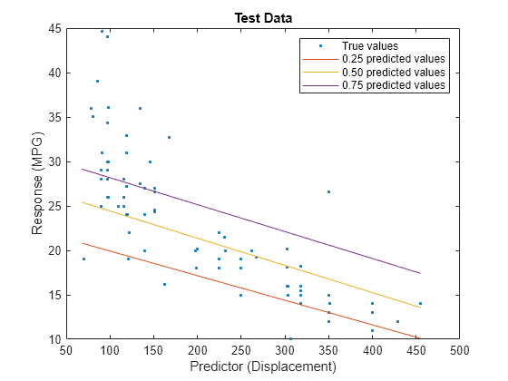
The red line shows the predictions for the 0.25 quantile, the yellow line shows the predictions for the 0.50 quantile, and the purple line shows the predictions for the 0.75 quantile. The blue points indicate the true test data values.

Notice that the quantile prediction lines do not cross each other.

Version History

Introduced in R2024b

R2025a: Store cross-validation optimization of hyperparameters

You can optimize the hyperparameters of a quantile linear regression model by specifying the OptimizeHyperparameters name-value argument in the call to fitrqlinear. A returned RegressionQuantileLinear object stores the cross-validation optimization of the hyperparameters in its HyperparameterOptimizationResults property.