Three-Parameter Weibull Distribution

Statistics and Machine Learning Toolbox™ uses a two-parameter Weibull Distribution with a scale parameter $$a$$ and a shape parameter $$b$$ in the probability distribution object WeibullDistribution and distribution-specific functions such as wblpdf and wblcdf. The Weibull distribution can take a third parameter. The three-parameter Weibull distribution adds a location parameter that is zero in the two-parameter case. If $$X$$ has a two-parameter Weibull distribution, then $$Y=X+c$$ has a three-parameter Weibull distribution with the added location parameter $$c$$.

The probability density function (pdf) of the three-parameter Weibull distribution becomes

$$f(x|a,b,c)=\{\begin{array}{ll}\frac{b}{a}{\left(\frac{x-c}{a}\right)}^{b-1}\exp (-{\left(\frac{x-c}{a}\right)}^b)& \text{if}x>c,\\ 0& \text{if}x\le c,\end{array}$$

where $$a$$ and $$b$$ are positive values, and $$c$$ is a real value.

If the scale parameter $$b$$ is less than 1, the probability density of the Weibull distribution approaches infinity as $$x$$ approaches $$c$$. The maximum of the likelihood function is infinite. The software might find satisfactory estimates in some cases, but the global maximum is degenerate when $$b<1$$.

This example shows how to find the maximum likelihood estimates (MLEs) for the three-parameter Weibull distribution by using a custom defined pdf and the mle function. Also, the example explains how to avoid the problem of a pdf approaching infinity when $$b<1$$.

Load Data

Load the carsmall data set, which contains measurements of cars made in the 1970s and early 1980s.

load carsmall

This example uses car weight measurements in the Weight variable.

Fit Two-Parameter Weibull Distribution

First, fit a two-parameter Weibull distribution to Weight.

pd = fitdist(Weight,'Weibull')

pd = 
  WeibullDistribution

  Weibull distribution
    A = 3321.64   [3157.65, 3494.15]
    B = 4.10083   [3.52497, 4.77076]

Plot the fit with a histogram.

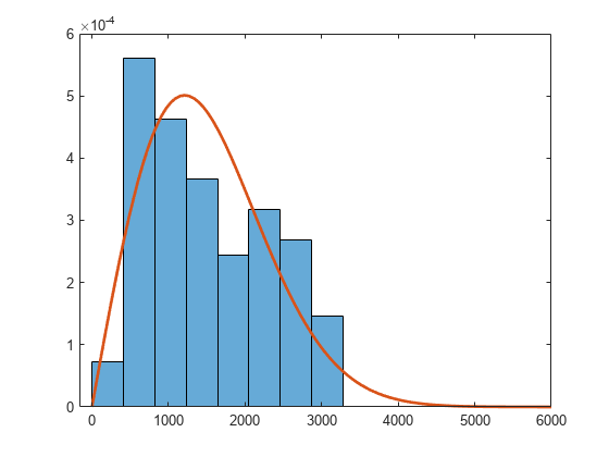
figure
histogram(Weight,8,'Normalization','pdf')
hold on
x = linspace(0,6000);
plot(x,pdf(pd,x),'LineWidth',2)
hold off

The fitted distribution plot does not match the histogram well. The histogram shows no samples in the region where Weight < 1500. Fit a Weibull distribution again after subtracting 1500 from Weight.

pd = fitdist(Weight-1500,'Weibull')

pd = 
  WeibullDistribution

  Weibull distribution
    A = 1711.75   [1543.58, 1898.23]
    B = 1.99963   [1.70954, 2.33895]

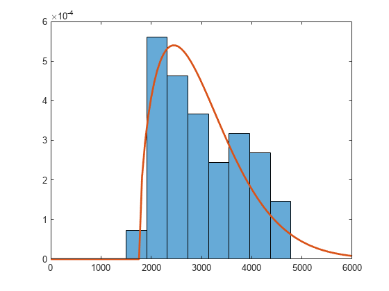
figure
histogram(Weight-1500,8,'Normalization','pdf')
hold on
plot(x,pdf(pd,x),'LineWidth',2)
hold off

The fitted distribution plot matches the histogram better.

Instead of specifying an arbitrary value for the distribution limit, you can define a custom function for a three-parameter Weibull distribution and estimate the limit (location parameter $$c$$).

Define Custom pdf for Three-Parameter Weibull Distribution

Define a probability density function for a three-parameter Weibull distribution.

f_def = @(x,a,b,c) (x>c).*(b/a).*(((x-c)/a).^(b-1)).*exp(-((x-c)/a).^b);

Alternatively, you can use the wblpdf function to define the three-parameter Weibull distribution.

f = @(x,a,b,c) wblpdf(x-c,a,b);

Fit Three-Parameter Weibull Distribution

Find the MLEs for the three parameters by using the mle function. You must also specify the initial parameter values (Start name-value argument) for the custom distribution.

try
    mle(Weight,'pdf',f,'Start',[1700 2 1500])
catch ME
    disp(ME)
end

  MException with properties:

    identifier: 'stats:mle:NonpositivePdfVal'
       message: 'Custom probability function returned negative or zero values.'
         cause: {}
         stack: [12x1 struct]
    Correction: []

mle returns an error because the custom function returns nonpositive values. This error is a typical problem when you fit a lower limit of a distribution, or fit a distribution with a region that has zero probability density. mle tries some parameter values that have zero density, and then fails to estimate parameters. In the previous function call, mle tries values of $$c$$ that are higher than the minimum value of Weight, which leads to a zero density for some points, and returns the error.

To avoid this problem, you can turn off the option that checks for invalid function values and specify the parameter bounds when you call the mle function.

Display the default options for the iterative estimation process of the mle function.

statset('mlecustom')

ans = struct with fields:
          Display: 'off'
      MaxFunEvals: 400
          MaxIter: 200
           TolBnd: 1.0000e-06
           TolFun: 1.0000e-06
       TolTypeFun: []
             TolX: 1.0000e-06
         TolTypeX: []
          GradObj: 'off'
         Jacobian: []
        DerivStep: 6.0555e-06
      FunValCheck: 'on'
           Robust: []
     RobustWgtFun: []
           WgtFun: []
             Tune: []
      UseParallel: []
    UseSubstreams: []
          Streams: {}
        OutputFcn: []

Override that default, using an options structure created with the statset function. Specify the FunValCheck field value as 'off' to turn off the validity check for the custom function values.

opt = statset('FunValCheck','off');

Find the MLEs of the three parameters again. Specify the iterative process option (Options name-value argument) and parameter bounds (LowerBound and UpperBound name-value arguments). The scale and shape parameters must be positive, and the location parameter must be smaller than the minimum of the sample data.

params = mle(Weight,'pdf',f,'Start',[1700 2 1500],'Options',opt, ...
    'LowerBound',[0 0 -Inf],'UpperBound',[Inf Inf min(Weight)])

params = 1×3
103 ×

    1.3874    0.0015    1.7581

Plot the fit with a histogram.

figure
histogram(Weight,8,'Normalization','pdf')
hold on
plot(x,f(x,params(1),params(2),params(3)),'LineWidth',2)
hold off

The fitted distribution plot matches the histogram well.

Fit Three-Parameter Weibull Distribution for $$b<1$$

If the scale parameter $$b$$ is less than 1, the pdf of the Weibull distribution approaches infinity near the lower limit $$c$$ (location parameter). You can avoid this problem by specifying interval-censored data, if appropriate.

Load the cities data set. The data includes ratings for nine different indicators of the quality of life in 329 US cities: climate, housing, health, crime, transportation, education, arts, recreation, and economics. For each indicator, a higher rating is better.

load cities

Find the MLEs for the seventh indicator (arts).

Y = ratings(:,7);
params1 = mle(Y,'pdf',f,'Start',[median(Y) 1 0],'Options',opt)

Warning: Maximum likelihood estimation did not converge.  Iteration limit exceeded.

params1 = 1×3
103 ×

    2.7584    0.0008    0.0520

The warning message indicates that the estimation does not converge. Modify the estimation options, and find the MLEs again. Increase the maximum number of iterations (MaxIter) and the maximum number of objective function evaluations (MaxFunEvals).

opt.MaxIter = 1e3;
opt.MaxFunEvals = 1e3;
params2 = mle(Y,'pdf',f,'Start',params1,'Options',opt)

Warning: Maximum likelihood estimation did not converge.  Function evaluation limit exceeded.

params2 = 1×3
103 ×

    2.7407    0.0008    0.0520

The iteration still does not converge because the pdf approaches infinity near the lower limit.

Assume that the indicators in Y are the values rounded to the nearest integer. Then, you can treat values in Y as interval-censored observations. An observation y in Y indicates that the actual rating is between y–0.5 and y+0.5. Create a matrix in which each row represents the interval surrounding each integer in Y.

intervalY = [Y-0.5, Y+0.5];

Find the MLEs again using intervalY. To fit a custom distribution to a censored data set, you must pass both the pdf and cdf to the mle function.

F = @(x,a,b,c) wblcdf(x-c,a,b);
params = mle(intervalY,'pdf',f,'cdf',F,'Start',params2,'Options',opt)

params = 1×3
103 ×

    2.7949    0.0008    0.0515

The function finds the MLEs without any convergence issues. This fit is based on fitting probabilities to intervals, so it does not encounter the problem of a density approaching infinity at a single point. You can use this approach only when converting data to an interval-censored version is appropriate.

Plot the results.

figure
histogram(Y,'Normalization','pdf')
hold on
x = linspace(0,max(Y));
plot(x,f(x,params(1),params(2),params(3)),'LineWidth',2)
hold off

The fitted distribution plot matches the histogram well.