Dense 3-D Reconstruction from Two Views Using RAFT Optical Flow
This example shows how to use optical flow to estimate the relative depth of a scene from two monocular images captured from different viewpoints. By tracking the motion of a pixel from one frame to another, optical flow provides dense correspondences between the pixels in two overlapping views of a scene. When you combine optical flow with known camera intrinsics and the estimated relative camera pose between the two views, you can triangulate and back-project a dense set of points in 3-D to obtain a dense depth image. You can then use the depth map to obtain a dense 3-D reconstruction in the form of a colored point cloud.
Two-view dense reconstruction is widely used in autonomous navigation, photogrammetry, and industrial automation. In photogrammetry, it is enables you to obtain 3-D elevation models from images taken by satellites or drones. In autonomous navigation tasks, you can use dense depth maps from visual sensors for obstacle avoidance, free-space mapping, and planning collision-free paths, often as a cheaper alternative to lidar sensors. In industrial automation, you can analyze a dense 3-D reconstruction of manufactured part to check for manufacturing defects.
This example computes the relative depth of a scene, resulting in a dense point cloud that is accurate up to scale. To resolve this scale ambiguity and obtain units like meters or centimeters, additional information is necessary. In mapping applications, you can obtain this information through geo-referencing using GPS or known camera altitudes. In other scenarios, you can use a known translation between the two views, similar to a known baseline in stereo vision.
The optical flow-based two-view dense reconstruction algorithm involves these steps:
Obtain Dense Point Correspondences Using Optical Flow from RAFT Model
Estimate Relative Camera Pose by Computing and Refining SIFT Point Matches
Refine Dense Point Correspondences from Optical Flow Using Geometric Constraints on SIFT Matches
Triangulate 3-D Points Using Refined Dense Correspondences
Compute Dense Depth Map by Back-Projecting Triangulated 3-D Points into First View
Create Colored Dense Point Cloud by Fusing Depth Map and RGB Colors of Scene
Set Up Data and Camera Parameters
Load the two images attached to this example. These images are a part of the "Office" video sequence from the TUM RGB-D Benchmark.
I1 = imread("1341848034.683883.png");
I2 = imread("1341848035.550852.png");
Create a cameraIntrinsics object to store the known camera intrinsic parameters.
focalLength    = [535.4 539.2];     % in pixels
principalPoint = [320.1 247.6];     % in pixels
imageSize      = size(I1,[1 2]);     % in pixels
intrinsics     = cameraIntrinsics(focalLength,principalPoint,imageSize);
Obtain Dense Point Correspondences Using Optical Flow from RAFT Model
Create opticalFlowRAFT Object
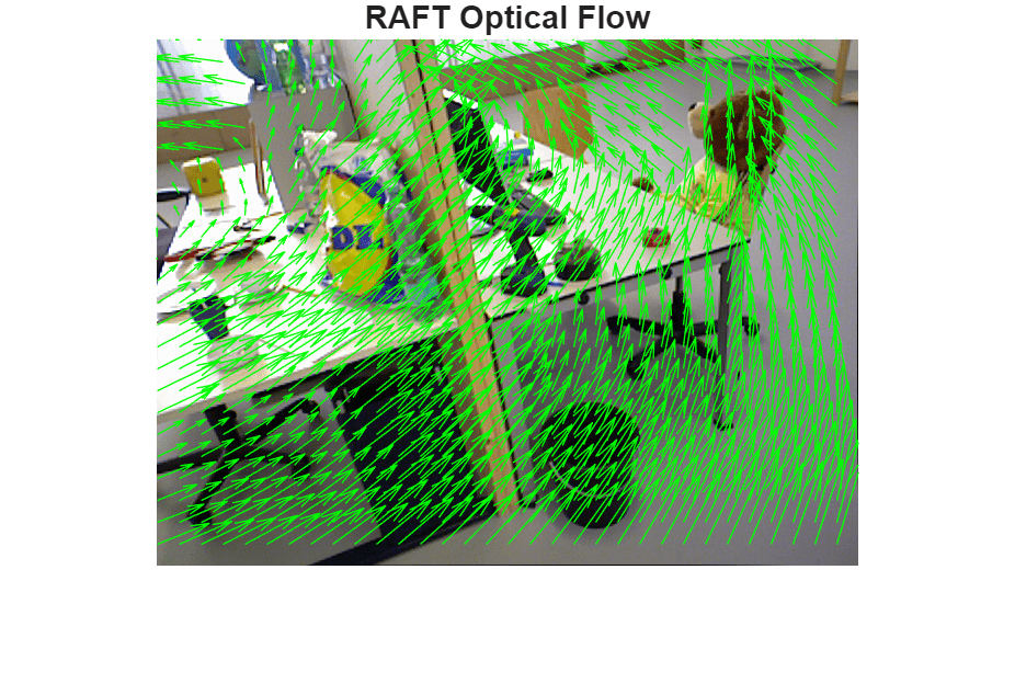
RAFT [1] is a state-of-the-art deep learning model for estimating optical flow that provides highly accurate results. It requires a GPU for optimal runtime performance. The quality of the dense reconstruction depends on the accuracy of dense pixel-to-pixel correspondences between two images. This example leverages the accurate predictions of dense optical flow from RAFT to obtain high-quality correspondences at every pixel.
raft = opticalFlowRAFT;
Compute Optical Flow on Two Frames
Display the pair of consecutive frames or views on which to estimate optical flow.
figure
montage({I1,I2},BorderSize=[2 2])
title("Two Views")
truesize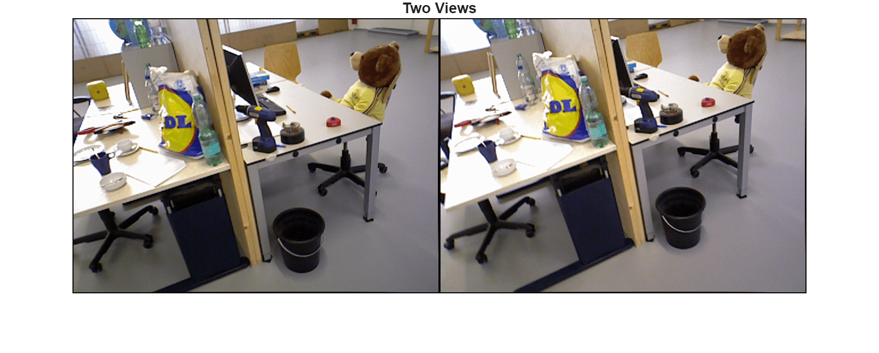
Visualize a red-cyan composite image of the two views to for better visualization of the relative camera motion.
J = stereoAnaglyph(I1,I2);
figure
imshow(J)
title("Red-Cyan Composite")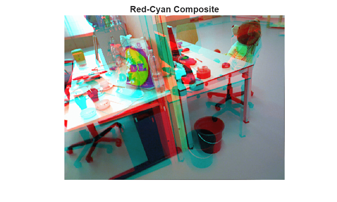
Estimate optical flow between the two frames.
estimateFlow(raft, I1);
flow = estimateFlow(raft, I2);
reset(raft);
Display the optical flow.
figure
imshow(I1)
hold on
plot(flow,DecimationFactor=[20 20],ScaleFactor=3.0,Color="green");
title("RAFT Optical Flow")
truesize
Filter Regions of Invalid Optical Flow
Apply a threshold on the optical flow magnitude to discard regions of uncertain optical flow, as well as points that lie outside of the image bounds. Optical flow vectors with magnitudes smaller than minFlowThreshold are considered invalid, as low-magnitude flow vectors are likely to have ambiguous orientation, and not be helpful in the subsequent 3-D triangulation stage.
A reasonable default value for this threshold is 1-2 pixels, which will discard flow vectors from regions that have less than 1-2 pixels of estimated movement.
minFlowThreshold = 2; % in pixelsCompute the target pixel positions for the pixels of I1 in I2, based on optical flow.
[H,W,~] = size(I1);
[X,Y] = meshgrid(1:W,1:H);
X2 = X + flow.Vx;
Y2 = Y + flow.Vy;
Compute the valid optical flow mask based on flow magnitude and image boundaries.
validFlow = X2>=1 & X2<=W & Y2>=1 & Y2<=H & flow.Magnitude > minFlowThreshold;
Compute the backward optical flow from I2 to I1. Use this to check the consistency of the optical flow computed in both directions between the two images.
estimateFlow(raft, I2);
flow2 = estimateFlow(raft, I1);
reset(raft);
Sample the components of backward flow, from image I2 to I1, at the forward-mapped pixel locations defined by (X2,Y2).
VxB = interp2(flow2.Vx, X2, Y2, 'linear', NaN);
VyB = interp2(flow2.Vy, X2, Y2, 'linear', NaN);
If the flows are consistent, the composition of the forward and backward optical flow vectors at corresponding points is close to zero.
fbFlowRes = hypot(flow.Vx + VxB, flow.Vy + VyB);
validFlow = validFlow & (fbFlowRes < minFlowThreshold);
Visualize the locations of valid optical flow using a blue overlay.
B = labeloverlay(I1,validFlow,Transparency=0.75);
figure
imshow(B)
title("Valid Optical Flow Regions")
truesize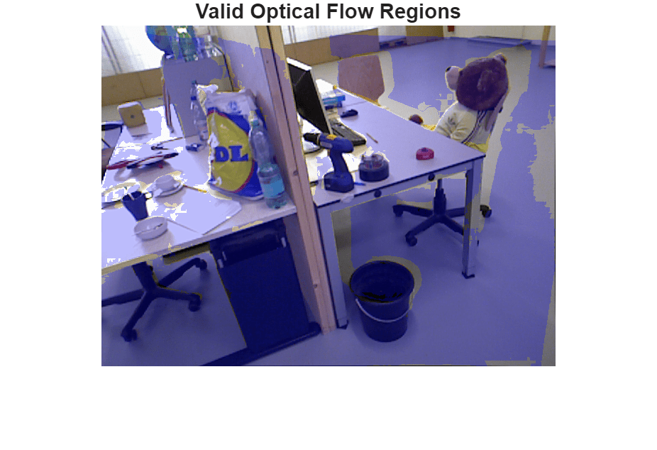
Observe that regions with very small flow vectors, and certain areas at the image boundaries, have been marked as invalid. The forward-backward flow consistency further rejects regions that are visible in one image but not in the other, as such regions also lead to invalid pixel correspondences between the two images.
Estimate Relative Camera Pose by Computing and Refining SIFT Point Matches
Estimating the relative camera pose between two views consists of these steps:
SIFT feature extraction and keypoint matching between the two views.
Estimation of the fundamental matrix, which captures the epipolar geometry between the two views.
Application of the epipolar constraints to refine the set of matched keypoints.
Estimation of the relative camera pose using the fundamental matrix and refined keypoint matches.
Keypoint Matching Using SIFT Features
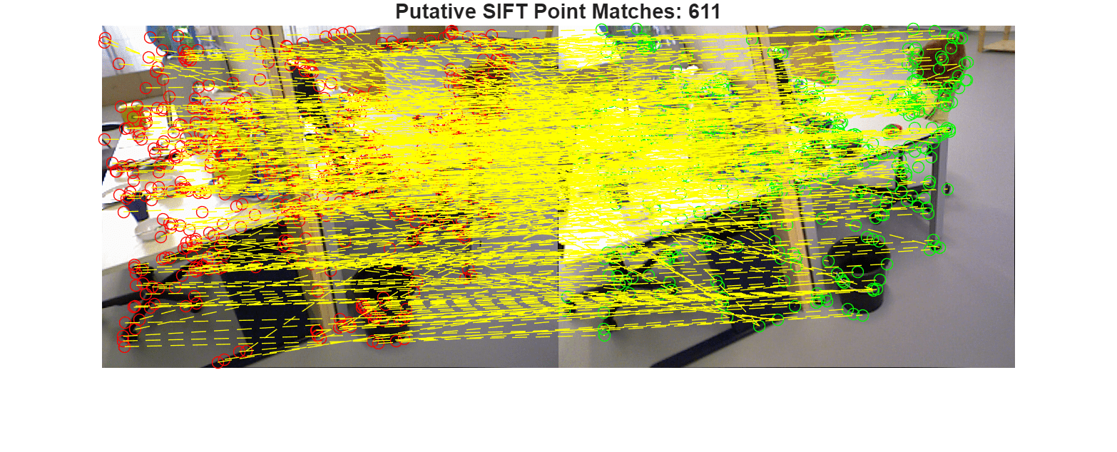
Use SIFT feature detection and matching to estimate the geometric transformation between the two frames. Optical flow matches, while densely covering the entire image, are too noisy for this purpose, which is why SIFT is preferable instead. Compute putative matches by exhaustively finding the nearest SIFT descriptor in the second image for each detected keypoint in the first image.
Use the ratio threshold to reject ambiguous matches. Increase this value to obtain more matches between features.
siftMaxRatio = 0.8;
0.8;Use the matching threshold for selecting the strongest matches. Increase the value of the matching threshold to obtain more matches between features.
siftMatchThreshold =  21;
21;Detect and match SIFT features between the two images.
points1 = detectSIFTFeatures(im2gray(I1));
[features1,validPoints1] = extractFeatures(im2gray(I1),points1);

points2 = detectSIFTFeatures(im2gray(I2));
[features2,validPoints2] = extractFeatures(im2gray(I2),points2);

indexPairs = matchFeatures(features1,features2,MaxRatio=siftMaxRatio, MatchThreshold=siftMatchThreshold);
matchedPoints1 = validPoints1(indexPairs(:,1));
matchedPoints2 = validPoints2(indexPairs(:,2));

figure
showMatchedFeatures(I1,I2,matchedPoints1,matchedPoints2,"montage",PlotOptions=["ro","go","y--"]);
title("Putative SIFT Point Matches: " + num2str(matchedPoints1.Count))
truesize
Compute the Fundamental Matrix
Estimate an essential matrix using the matched points and known camera intrinsics, and use this to compute the fundamental matrix. When camera intrinsics are known, this is more numerically stable than directly estimating the fundamental matrix from point matches, and also results in better accuracy.
A robust estimate of the essential matrix between the two images is derived using the M-estimator Sample Consensus (MSAC) algorithm, a variant of the RANSAC algorithm [2]. Specify the parameters of the RANSAC algorithm which control the tradeoff between speed and accuracy.
Setting a larger number of trials for RANSAC allows the algorithm to run longer until it finds a higher-quality solution, at the cost of longer runtime.
ransacMaxNumTrials = 1e3;
Setting a larger value of maximum allowed distance allows the algorithm to converge faster, but can also result in a lower quality estimation.
ransacMaxDist = 4;
Estimate the essential matrix E and use this to obtain the fundamental matrix F.
[E, inliers] = estimateEssentialMatrix( ...
    matchedPoints1, matchedPoints2, intrinsics,MaxNumTrials=1e3, MaxDistance=ransacMaxDist);
F = intrinsics.K'\ E /intrinsics.K;
Refine SIFT keypoint matches
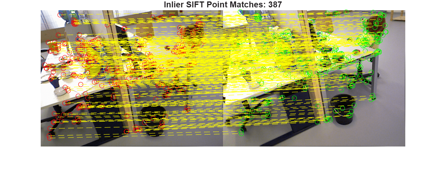
Prune the set of matched points based on how well they correspond to the epipolar geometric transformation defined by the estimated fundamental matrix.
inlierPoints1 = matchedPoints1(inliers);
inlierPoints2 = matchedPoints2(inliers);
Display the inlier SIFT matches that fit the estimated epipolar geometry of the fundamental matrix.
figure
showMatchedFeatures(I1,I2,inlierPoints1,inlierPoints2,"montage",PlotOptions=["ro","go","y--"]);
title("Inlier SIFT Point Matches: " + num2str(nnz(inliers)));
truesize
Compute Relative Camera Pose
Use known camera intrinsics, the estimated fundamental matrix and the geometrically verified inlier matches to compute the relative pose between the two camera positions.
relPose = estrelpose(F,intrinsics,inlierPoints1,inlierPoints2);
Display the estimated relative pose, which comprises of a rotation and a translation in three dimensions. Note that the estimated translation will be accurate up to an unknown scale factor.
disp(relPose)
  rigidtform3d with properties:

    Dimensionality: 3
       Translation: [-0.8912 0.4152 -0.1824]
                 R: [3×3 double]

                 A: [ 0.9972   -0.0534    0.0526   -0.8912
                      0.0530    0.9986    0.0085    0.4152
                     -0.0530   -0.0057    0.9986   -0.1824
                           0         0         0    1.0000]
Triangulate 3-D Points from Refined Dense Correspondences
Compute densely matched pixels between the two images based on validFlow.
matchedDensePts1 = single([X(validFlow), Y(validFlow)]);
matchedDensePts2 = [X2(validFlow), Y2(validFlow)];
Assume the first camera to be at the origin of a 3D world coordinate system. The pose of the second camera is then the relative camera pose estimated earlier.
cam1Pose = rigidtform3d();
cam2Pose = relPose;
Combine the intrinsics and camera extrinsics into a single camera projection matrix for each of the two images.
camProj1 = cameraProjection(intrinsics,pose2extr(cam1Pose));
camProj2 = cameraProjection(intrinsics,pose2extr(cam2Pose));
Use the camera intrinsics, relative camera pose and dense matched points from RAFT optical flow to triangulate the matched 2D points into 3D points.
[points3D, reprojectionErr, validPoints3D]  = triangulate(...
    matchedDensePts1, matchedDensePts2, camProj1, camProj2);
points3D = points3D(validPoints3D,:);
reprojectionErr = reprojectionErr(validPoints3D);
Visualize Triangulated Points and Determine Maximum Depth Threshold
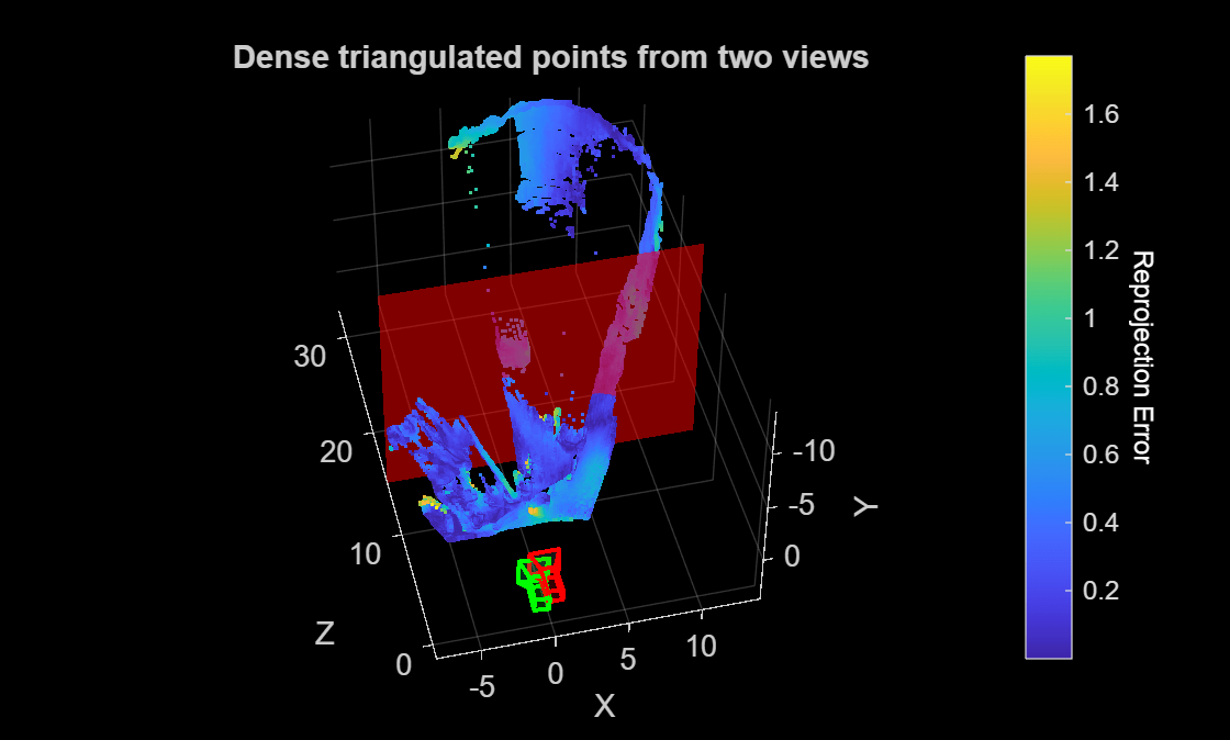
Visualize the 3D points and the camera positions.
figure
h1 = pcshow(points3D, reprojectionErr, VerticalAxis="y", VerticalAxisDir="down");
xlabel("X")
ylabel("Y")
zlabel("Z")

hold on
plotCamera(AbsolutePose=cam1Pose,Size=1,Opacity=0.1,Color="red");
plotCamera(AbsolutePose=cam2Pose,Size=1,Opacity=0.1,Color="green");

cb = colorbar;
ylabel(cb,"Reprojection Error",Rotation=270,Color="white")

title("Dense triangulated points from two views")
Use the slider to determine the maximum valid depth. Points that are extremely far away from the camera are usually error prone and can be clipped from the final reconstruction by setting this threshold.
maxDepthThreshold =15; hPlane = constantplane(h1,"z",maxDepthThreshold,FaceColor="red",FaceAlpha=0.5); hold off
Compute Dense Depth Map by Back-Projecting Triangulated 3-D Points into First View
Compute depth at valid pixel locations in the coordinate frame of the first image.
% Transform the triangulated 3D points to the reference camera frame
% which is assumed to be at the origin.
Z = points3D(:,3);

% Filter by maximum depth threshold
validDepth = Z > 0 & Z < maxDepthThreshold;

% Depth map combining valid locations of flow and depth
depthMap = nan(H,W);
idxValid = find(validFlow);
idxValid = idxValid(validDepth);
Z = Z(validDepth);
depthMap(idxValid) = Z;

% Visualize depth map in log-scale for better contrast
figure
colormap(gray)
imagesc(log(1 + depthMap))
axis image
colorbar
title("Depth Map (log-scale)")
truesize
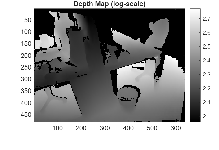
The depth map captures the fine details in the scene, such as sharp boundaries at the desk edges, the bucket and the teddy bear. Regions of invalid depth, such as being too far away from the camera or due to optical flow uncertainty, are marked as NaNs and appear as black pixels in the visualized log-scaled depth map.
Create Colored Dense Point Cloud by Fusing Depth Map and RGB Image
Create a colored point cloud by mapping the pixel values in the image to their corresponding triangulated 3D points.
% Valid pixel positions
u = X(validFlow);
v = Y(validFlow);
u = u(validDepth);
v = v(validDepth);

% Get RGB colors at those pixel positions
linearIdx = sub2ind([H,W], v, u);
R = I1(:,:,1);
G = I1(:,:,2);
B = I1(:,:,3);
colors = [R(linearIdx), G(linearIdx), B(linearIdx)];

% Valid 3D points
validDepthPoints = points3D(validDepth,:);

% Create a pointCloud object using colors and 3D point locations
ptCloud = pointCloud(validDepthPoints, Color=colors);

% Visualize the point cloud
figure
ax = pcshow(ptCloud,VerticalAxis="y", VerticalAxisDir="down");
xlabel("X")
ylabel("Y")
zlabel("Z")
title("Dense Colored Point Cloud from Two Views")

view(0,-80)
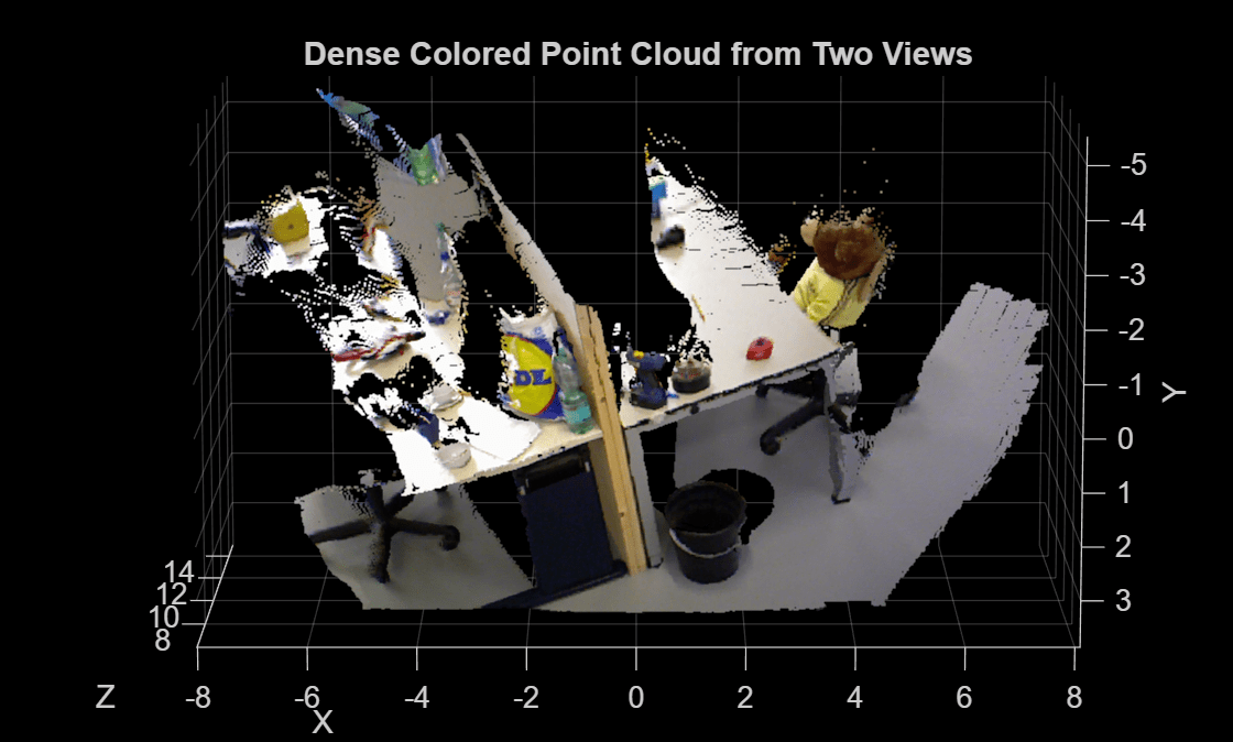
The resulting point cloud provides a dense 3D reconstruction of the scene, up to an unknown scale factor, using two views taken by a calibrated monocular camera. For more information on metric reconstruction of the scene, see Structure from Motion from Two Views.
References
[1] Teed, Z., & Deng, J. "RAFT: Recurrent All-Pairs Field Transforms for Optical Flow." European Conference in Computer Vision, 2020.
[2] Tordoff, B & Murray, DW. "Guided Sampling and Consensus for Motion Estimation." European Conference in Computer Vision, 2002.
[3] Schönberger, J. L. & Frahm J.-M., "Structure-from-Motion Revisited," IEEE Conference on Computer Vision and Pattern Recognition 2016.
See Also
opticalFlowRAFT | detectSIFTFeatures | estimateEssentialMatrix | estrelpose