Using Gabor-Based Time-Frequency Filtering for Audio Source Separation

Since R2025a

This example uses:

This example shows how to isolate a speech signal using a binary mask with the discrete Gabor transform (DGT). You compare results with those obtained using the short-time Fourier transform (STFT). Gabor-based time-frequency filtering enables precise signal manipulation in the time-frequency domain.

Import Data

Load audio files containing male and female speech sampled at 4 kHz. These audio files are from the example Cocktail Party Source Separation Using Deep Learning Networks (Audio Toolbox). The duration of each file is about 20 seconds. Listen to the audio files individually for reference.

[mSpeech,Fs] = audioread("MaleSpeech-16-4-mono-20secs.wav");
soundsc(mSpeech,Fs)

[fSpeech] = audioread("FemaleSpeech-16-4-mono-20secs.wav");
soundsc(fSpeech,Fs)

Create Signal

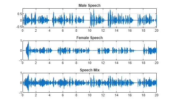
Combine the two speech sources. Ensure the sources have equal power in the mix. Scale the mix so that its maximum amplitude is one.

mSpeech = mSpeech/norm(mSpeech);
fSpeech = fSpeech/norm(fSpeech);

ampAdj = max(abs([mSpeech;fSpeech]));
mSpeech = mSpeech/ampAdj;
fSpeech = fSpeech/ampAdj;

mix = mSpeech + fSpeech;
mix = mix./max(abs(mix));

Visualize the original and mixed signals.

tm = (0:numel(mSpeech)-1)/Fs;
tiledlayout(3,1)
nexttile
plot(tm,mSpeech)
title("Male Speech")
grid on
nexttile
plot(tm,fSpeech)
title("Female Speech")
grid on
nexttile
plot(tm,mix)
title("Speech Mix")
grid on

Figure contains 3 axes objects. Axes object 1 with title Male Speech contains an object of type line. Axes object 2 with title Female Speech contains an object of type line. Axes object 3 with title Speech Mix contains an object of type line.

Listen to the mixed speech signal.

soundsc(mix,Fs)

Time-Frequency Filtering Using STFT

Obtain STFT

Time-frequency filtering with the short-time Fourier transform involves inverting the transform. To ensure perfect reconstruction of nonmodified spectra using the ISTFT, the analysis window and the overlap must satisfy the Constant Overlap-Add (COLA) Constraint. Use the function hann (Signal Processing Toolbox) to specify a Hann window of length 128 and an overlap of 96 samples. Use the function iscola (Signal Processing Toolbox) to confirm the window and overlap satisfy the constraint.

winLen = 128;
win = hann(winLen,"periodic");
overlapLen = 96;
fprintf("Does window satisfy cola condition? %d\n",iscola(win,overlapLen))

Does window satisfy cola condition? 1

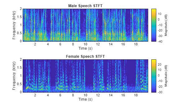
Use the function stft (Signal Processing Toolbox) to obtain the one-sided STFT of the male and female signals. Specify 128 DFT points.

frqRng = "onesided";
numBin = 128;
Sm = stft(mSpeech, ...
    Window=win, ...
    OverlapLength=overlapLen, ...
    FFTLength=numBin, ...
    FrequencyRange=frqRng);

Sf = stft(fSpeech, ...
    Window=win, ...
    OverlapLength=overlapLen, ...
    FFTLength=numBin, ...
    FrequencyRange=frqRng);

Visualize the magnitude of the STFT of the two signals.

figure
tiledlayout(2,1)
nexttile
stft(mSpeech, Fs, ...
    Window=win, ...
    OverlapLength=overlapLen, ...
    FFTLength=numBin, ...
    FrequencyRange=frqRng)
title("Male Speech STFT")
nexttile
stft(fSpeech, Fs, ...
    Window=win, ...
    OverlapLength=overlapLen, ...
    FFTLength=numBin, ...
    FrequencyRange=frqRng)
title("Female Speech STFT")

Figure contains 2 axes objects. Axes object 1 with title Male Speech STFT, xlabel Time (s), ylabel Frequency (kHz) contains an object of type image. Axes object 2 with title Female Speech STFT, xlabel Time (s), ylabel Frequency (kHz) contains an object of type image.

Create Binary Mask Using STFT

Use the STFT of both signals to create a binary mask. A true value identifies a time-frequency bin where the magnitude of the STFT of the male signal is greater than or equal to the corresponding bin in the STFT of the female signal.

stftBmask = abs(Sm) >= abs(Sf);

Reconstruct Male Speech

Apply the binary mask to the STFT of the mixed signal. Use the function istft (Signal Processing Toolbox) to invert the result.

[S_mix,F] = stft(mix, ...
    Window=win, ...
    OverlapLength=overlapLen, ...
    FFTLength=numBin, ...
    FrequencyRange=frqRng);

stftmSpeechRec = istft(S_mix.*stftBmask, ...
    Window=win, ...
    OverlapLength=overlapLen, ...
    FFTLength=numBin, ...
    FrequencyRange=frqRng);

Time-Frequency Filtering Using DGT

Obtain DGT

Use the dgt function to obtain the one-sided DGT of the male and female signals. Use the same parameters used for the STFT. Note that the hop length is the difference between the window length and overlap.

Dm = dgt(mSpeech, ...
    WindowLength=winLen, ...
    HopLength=winLen-overlapLen, ...
    NumFrequencyBins=numBin, ...
    FrequencyRange=frqRng);

Df = dgt(fSpeech, ...
    WindowLength=winLen, ...
    HopLength=winLen-overlapLen, ...
    NumFrequencyBins=numBin, ...
    FrequencyRange=frqRng);

Visualize the magnitude of the DGT of both signals.

figure
tiledlayout(2,1)
nexttile
dgt(mSpeech, ...
    SampleRate=Fs, ...
    WindowLength=winLen, ...
    HopLength=winLen-overlapLen, ...
    NumFrequencyBins=numBin, ...
    FrequencyRange=frqRng)
title("Male Speech DGT")
nexttile
dgt(fSpeech, ...
    SampleRate=Fs, ...
    WindowLength=winLen, ...
    HopLength=winLen-overlapLen, ...
    NumFrequencyBins=numBin, ...
    FrequencyRange=frqRng)
title("Female Speech DGT")

Figure contains 2 axes objects. Axes object 1 with title Male Speech DGT, xlabel Time (s), ylabel Frequency (kHz) contains an object of type image. Axes object 2 with title Female Speech DGT, xlabel Time (s), ylabel Frequency (kHz) contains an object of type image.

Create Binary Mask Using DGT

Use the DGT of both signals to create a binary mask. For the STFT, you created a mask that identified the STFT coefficients to include for the inverse transform. The tffilt function expects the binary mask to identify the DGT coefficients to filter out before reconstruction. Therefore, to reconstruct the male signal, create a mask where a true value identifies a time-frequency bin where the magnitude of the DGT of the female signal is greater than the corresponding bin in the DGT of the male signal.

dgtBmask = abs(Df) > abs(Dm);

Reconstruct Male Speech

Use the binary mask in tffilt to reconstruct the male signal. To apply the mask directly to the DGT of the input signal, specify the "gm" time-frequency filtering method.

dgtmSpeechRec = tffilt(dgtBmask,mix, ...
    WindowLength=winLen, ...
    HopLength=winLen-overlapLen, ...
    NumFrequencyBins=numBin, ...
    FrequencyRange=frqRng, ...
    Method="gm");

Compare Reconstructions

To compare the original male signal with the STFT- and DGT-based reconstructions, compute these two metrics for each reconstruction.

Signal-to-interference ratio (SIR) — The higher the SIR, the better the performance. To compute this metric, use the helper function helperComputeSIR. The source for this function is listed in the appendix.
Itakura-Saito distance (ISD) — The lower the ISD, the better the performance. To compute this metric, use the helper function helperComputeISD. The source for this function is listed in the appendix. The Itakura–Saito distance (or divergence) quantifies the difference between an original spectrum and its approximation. While not inherently a perceptual measure, the metric is designed to capture perceptual (dis)similarity. For more information about the ISD, see [5].

sirBefore = helperComputeSIR(mSpeech,mix);
sirSTFT = helperComputeSIR(mSpeech,stftmSpeechRec);
sirDGT = helperComputeSIR(mSpeech,dgtmSpeechRec);
isdBefore = helperComputeISD(mSpeech,mix);
isdSTFT = helperComputeISD(mSpeech,stftmSpeechRec);
isdDGT = helperComputeISD(mSpeech,dgtmSpeechRec);

T = table(round([sirBefore;sirSTFT;sirDGT]), ...
    round([isdBefore;isdSTFT;isdDGT]), ...
    variableNames=["SIR (dB)","ISD"], ...
    RowNames=["Before","STFT","TFFILT"])

T=3×2 table
              SIR (dB)     ISD 
              ________    _____

    Before        1       21026
    STFT          6       26174
    TFFILT       12        6365

Summary

In this example, you learned how to isolate a speech signal by using a binary mask with the DGT. The tffilt function performed the time-frequency filtering by applying the binary mask directly to the DGT of the mixed signal and reconstructing the result using the inverse DGT. The function supports two additional filtering methods. Both methods involve Gabor multipliers, linear operators that apply a pointwise product with a time-frequency transfer function, or mask. Time-frequency filtering using Gabor multipliers offers a robust and adaptable solution for precise signal manipulation. You can also provide tffilt a collection of binary masks to apply sequentially to the DGT before reconstructing the filtered signal.

Appendix

helperComputeSIR

function s = helperComputeSIR(x,xh)
% helperComputeSIR Compute signal-to-interference ratio
% This function is only intended to support this wavelet example.
% It may change or be removed in a future release.

s = 20*log10(norm(x,2)/norm(xh-x,2));
end

helperComputeISD

function dis = helperComputeISD(x,xh)
% helperComputeISD Itakura-Saito distance
% This function is only intended to support this wavelet example.
% It may change or be removed in a future release.

arguments
    x  {mustBeFloat,mustBeVector}
    xh {mustBeFloat,mustBeVector}
end
validateattributes(xh,{'numeric'},{'numel',length(x)})

rdtPropto = zeros("like",real(x([]))) + zeros("like",real(xh([])));
xc = reshape(cast(x,"like",rdtPropto),[],1);
xhc = reshape(cast(xh,"like",rdtPropto),[],1);

p = abs(fft(xc));
ph = abs(fft(xhc));

% DIS(P(w),Ph(w)) = int_(-pi)^(pi)[P(w)/Ph(w)-log(P(w)/Ph(w))-1]dw/2*pi
z = p./(ph+eps(ph));
dis = sum(z - log(z)) - length(z);

end

References

[1] Krémé, A. Marina, Valentin Emiya, Caroline Chaux, and Bruno Torrésani. “Time-Frequency Fading Algorithms Based on Gabor Multipliers.” IEEE Journal of Selected Topics in Signal Processing 15, no. 1 (January 2021): 65–77. https://doi.org/10.1109/JSTSP.2020.3045938.

[2] Mallat, S.G. and Zhifeng Zhang. “Matching Pursuits with Time-Frequency Dictionaries.” IEEE Transactions on Signal Processing 41, no. 12 (December 1993): 3397–3415. https://doi.org/10.1109/78.258082.

[3] Søndergaard, Peter. “An Efficient Algorithm for the Discrete Gabor Transform Using Full Length Windows.” In SAMPTA ’09 International Conference on SAMPling Theory and Applications, edited by Laurent Fesquet and Bruno Torresani, 223–26. Marseille, France, 2009. https://hal.science/hal-00495456/file/SampTAProceedings.pdf.

[4] Halko, N., P. G. Martinsson, and J. A. Tropp. “Finding Structure with Randomness: Probabilistic Algorithms for Constructing Approximate Matrix Decompositions.” SIAM Review 53, no. 2 (January 2011): 217–88. https://doi.org/10.1137/090771806.

[5] Itakura, F., and S. Saito. “Analysis Synthesis Telephony Based on the Maximum Likelihood Method.” In Proc. 6th International Congress on Acoustics, C17–20. Los Alamitos, CA, 1968.

Using Gabor-Based Time-Frequency Filtering for Audio Source Separation

Import Data

Create Signal

Time-Frequency Filtering Using STFT

Obtain STFT

Create Binary Mask Using STFT

Reconstruct Male Speech

Time-Frequency Filtering Using DGT

Obtain DGT

Create Binary Mask Using DGT

Reconstruct Male Speech

Compare Reconstructions

Summary

Appendix

References

See Also

Topics