Viewing CWT Decomposition of Image in Wavelet Image Analyzer

When you load an image into Wavelet Image Analyzer, the app immediately decomposes the image using the discrete wavelet transform (DWT). Wavelet Image Analyzer can also decompose an image using the continuous wavelet transform (CWT). You can decompose the image using the CWT by clicking Add on the Analyzer tab and selecting CWT. The app decomposes the image using default wavelet parameters.

Transform and Visualization Parameters

After you generate the CWT decomposition of an image, Wavelet Image Analyzer switches to the CWT tab. On the tab, you can change the transform parameters that the app uses to generate the decomposition. Changing any transform parameter enables the Compute CWT button. Click the button to apply the changes.

The 2-D CWT is a representation of 2-D data (image data) in four variables: dilation (or scale), rotation, and position. Scale and rotation are real-valued scalars and position is a 2-D vector with real-valued elements. You can control how to display the decomposition in Wavelet Image Analyzer:

• Fix a rotation and vary the scales

• Fix a scale and vary the rotations

If the decomposition is complex valued, you can display either the magnitude and phase or real and imaginary parts of the decomposition.

Tab Sections

• Wavelet — Specify the wavelet and normalization. You can specify either L1 or L2 normalization. You can choose an isotropic or anisotropic wavelet. Isotropic wavelets are not sensitive to the orientation of features. Anisotropic wavelets are sensitive to the orientation.

  • Isotropic — Gaussian, and Marr

  • Anisotropic — Cauchy, Endstop, and Morlet

  Note

  The Marr wavelet is real valued. If you use the Marr wavelet in the 2-D CWT of an image, the decomposition is also real valued.

• Scale — Scales to use in the CWT.

  • Max Scale — Specify a value in pixels. The app determines the logarithmically spaced scales. The support of the dilated wavelet at all scales does not exceed Max Scale pixels. By default, Max Scale is min(size(img,[1 2])), where img is the image.

  • Specify Scales — Specify scales to use in the CWT. Scales must be greater than or equal to 1.

  For more information, see CWT Scales in Wavelet Image Analyzer.

  Note

  If necessary, Wavelet Image Analyzer zero-pads the image so that there is at least one scale in the decomposition.

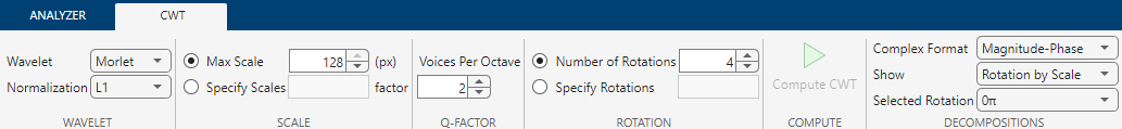
• Q-Factor — Specify the number of voices per octave to use for the CWT.

• Rotation — Rotation angles to use in the CWT.

  • Number of Rotations — Number of angles to evenly distribute in the interval [0, 2π), specified as a positive integer ≤ 15. If Number of Rotations is N, then the angles are 2*pi/N*[0:N-1].

  • Specify Rotations — User-specified angles in radians.

• Decompositions — How to display the decomposition.

  • Complex Format — For a complex-valued decomposition, choose either Magnitude-Phase or Real-Imaginary.

  • Show — To display the decomposition by scales for a specific rotation, select Rotation by Scale, and then select the desired rotation from the Selected Rotation list.

    To display the decomposition by angles for a specific scale, select Scale by Angle, and then select the desired rotation from the Selected Scale list.

Note

If you select an isotropic wavelet, parameters that involve rotations are disabled.

Interacting with Decomposition Images

To show or hide a row in the Decompositions pane, select or clear the check box in the corresponding row in the Scale Selection or Rotation Selection pane.

To hide all the plots in a row or column in the Decompositions pane, right-click a plot in that row or column and select the desired action. You can restore all plots, right-click anywhere in the Decompositions pane and select Show complete decomposition.

Visualize CWT Decomposition of Image and Export Results

This example shows how to visualize the continuous wavelet transform (CWT) decomposition of an image and recreate the results in the workspace.

Import Data

You can import an image from your workspace or a file into Wavelet Image Analyzer. Read the RGB image of the hexagon into your workspace.

hexa = imread("hexagon.jpg");

Visualize CWT Decomposition

Open Wavelet Image Analyzer.

1. On the Analyzer tab, click Import to open the Import Images dialog box. The dialog box lists all the workspace variables the app can process, along with their dimensions.

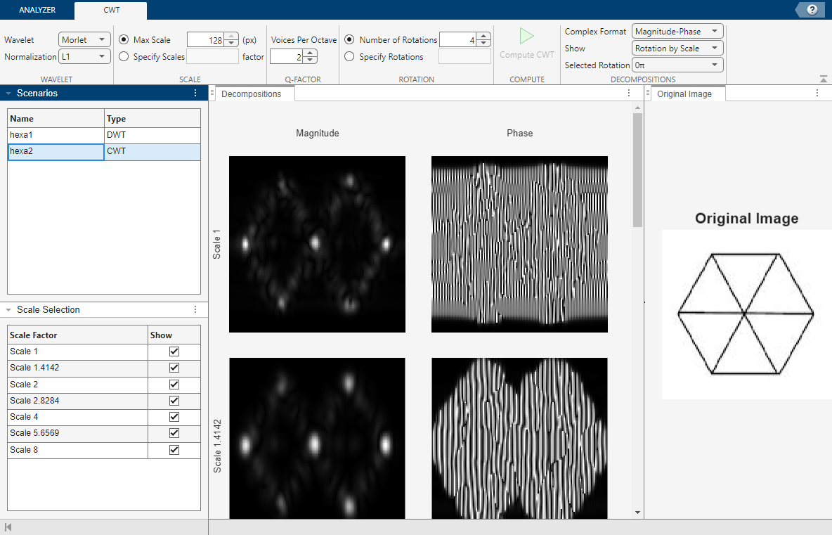
2. Select hexa and click Import. By default, a four-level discrete wavelet transform (DWT) decomposition of the image appears. The scenario name is hexa1.

3. On the Analyzer tab, click Add > CWT.

A CWT decomposition of the image appears. The app switches to the CWT tab. The scenario name is hexa2. The app computes the CWT using the Morlet wavelet with a Q-factor, or voices per octave, of 2, and four equispaced rotation angles. In the Decompositions pane, the app shows the magnitudes and phases of the coefficients at all scales for the rotation angle 0 radians.

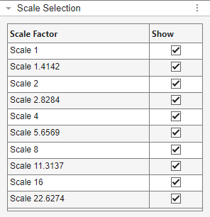
The Scale Selection pane lists the scale factors used in the CWT. The scale factors are logarithmically spaced. To learn how the app determines the scales, see CWT Scales in Wavelet Image Analyzer.

Change Transform Parameters

By default, the app shows the decomposition at all scales for a given angle, 0 radians. If, in the Decompositions section of the toolstrip, you set Show to Scale by Angle, and inspect the plots at all angles, you will note that only the horizontal features of the hexagon are prominent in the magnitude plots.

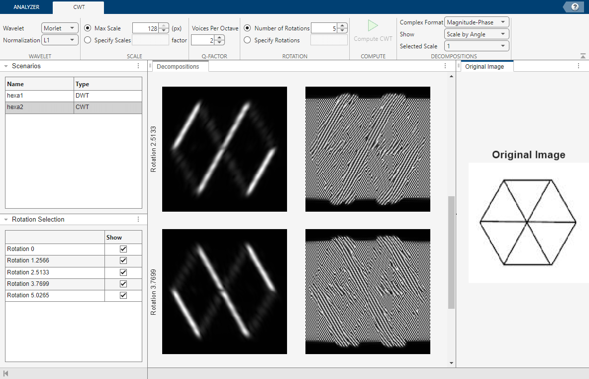
Set Number of Rotations to 5 and compute the CWT. Set Show to Scale by Angle. The diagonal features are prominent at the rotation angles $$4\pi /5$$ and $$6\pi /5$$. However, the horizontal features are not visible at any angles. With Wavelet Image Analyzer, you can explore how features are captured by the CWT by increasing the number of angles.

Export Results

You can either export the CWT decomposition to your workspace or generate a script to reproduce the results.

To generate a script to recreate the hexa2 decomposition in your workspace, in the Analyzer tab, select Export > Generate MATLAB Script. An untitled script opens in your editor with the following executable code. You can save the script as is or modify it to apply the same compression to other signals. Run the code. The output of the cwtft2 function, hexa2_CWT, is a structure. See cwtft2 for a description of the structure.

If you export the CWT decomposition of the scenario scenarioName, the name of the exported workspace variable is scenarioName_CWT. The variable is a structure with one field: cwtStruct. This structure is identical to hexa2_CWT.

% Define wavelet parameters
wname = "morlet";      % Name
k0 = 2.60258056913715; % Center frequency
sigma = 3.46442623512; % Standard deviation

waveletStruct.name = wname;
waveletStruct.param = {k0, sqrt(sigma)};

% Define 2-D CWT parameters
scales = [1 1.4142135623731 2 2.82842712474619 4 5.65685424949238 8];
angles = [0*pi 2*pi/5 4*pi/5 6*pi/5 8*pi/5];
nm = "L1";

% Perform the decomposition using CWTFT2 to obtain the 2-D CWT structure
hexa2_CWT = cwtft2(hexa,Wavelet=waveletStruct,Scales=scales, ...
    Angles=angles,Norm=nm);

% For an image of size M-by-N-by-K, where K is 1 or 3, CWT coefficients
% are returned in the structure field hexa2_CWT.cfs as an
% M-by-N-by-K-by-Nscales-by-Nangles array, where:
% * Nscales is the number of scales.
% * Nangles is the number of angles.

% To view the magnitude of the coefficients with the IMSHOW function,
% try scaling them with the WCODEMAT function. For example:
% >> imshow(uint8(wcodemat(abs(hexa2_CWT.cfs(:,:,:,1,1)),255)))

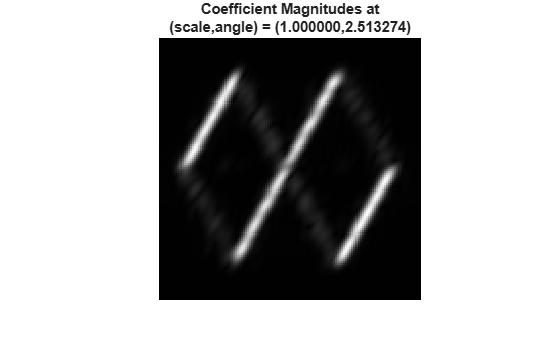
View the magnitude of the coefficients at scale 1 and angle $$4\pi /5$$ and compare with the plot in the app. Confirm they are identical.

scaleInd = 1;
angleInd = 3;
imshow(uint8(wcodemat(abs(hexa2_CWT.cfs(:,:,:,scaleInd,angleInd)),255)))
str = sprintf("Coefficient Magnitudes at\n(scale,angle) = (%f,%f)", ...
    scales(scaleInd),angles(angleInd));
ax = gca;
ax.PositionConstraint = "outerposition";
title(str)

CWT Scales in Wavelet Image Analyzer

The 2-D CWT of an image is a function of three variables: position, rotation, and scale. In Wavelet Image Analyzer, you set, among other transform parameters, the rotation angles and scales. For both variables, you can either have the app choose specific values to use in the CWT, or you can specify them yourself. This example shows how Wavelet Image Analyzer determines the scales.

To have Wavelet Image Analyzer determine the scales, you set Max Scale to a value in pixels. The app chooses the scales based on:

• Max Scale

• Size of the wavelet support in pixels at scale 1, for example, undilated

• Number of voices per octave

The app first determines the spatial support of the wavelet. Then, based on the support and number of voices per octave, the app obtains the scales. The scales are logarithmically spaced, and such that the support of the dilated wavelet at all scales does not exceed Max Scale. Keep in mind that the app only allows scales greater than or equal to 1. You can never shrink the spatial support of the wavelet.

By default, Max Scale is min(size(img,[1 2])), where img is the input image. In the app, you cannot set Max Scale to a value greater than min(size(img,[1 2])). This constraint ensures that the dilated wavelet support will never exceed the image dimensions. If necessary, Wavelet Image Analyzer zero-pads the image so that there is at least one scale in the decomposition.

Determining Wavelet Support

To determine the wavelet support, the app first obtains the wavelet at scale 1. Next, the app:

1. Normalizes this 2-D function into a probability density function (PDF).

2. Obtains the marginal PDFs in the X and Y spatial variables.

3. Determines the 0.005 and 0.995 points on the marginal distributions. The interval contains 0.99 of the probability.

The app uses the width of the maximum of these two intervals as the support of the wavelet.

Illustration — Gaussian Wavelet

Load an image. Set maxScale to the minimum of the row and column dimension sizes.

img = imread("hexagon.jpg");
maxScale = min(size(img,[1 2]));

Determine Support

For the Gaussian wavelet in Wavelet Image Analyzer, the following code defines the wavelet in the spatial angular frequency domain. This example uses a square grid consisting of 129 points in the X and Y directions.

omegax = 2*pi.*(-64/129:1/129:64/129);
omegay = 2*pi.*(-64/129:1/129:64/129);
[omegax,omegay] = meshgrid(omegax,omegay);
psihat = 1i.*(omegax+1i.*omegay).*exp(-(omegax.^2+omegay.^2)./2);

Obtain the centered wavelet in the spatial domain.

psi = ifftshift(ifft2(psihat));

For this wavelet, obtain a support of approximately 5.4. Plot the magnitude of the wavelet in the spatial domain. The magnitude of the wavelet is centered at (1,1). Show the estimated extent of the support in the X-direction around the center.

x = -64:64;
y = -64:64;
surf(x,y,abs(psi))
view(-1,37)
shading interp
xlim([-10 10])
ylim([-10 10])
hold on
plot([1-5.4/2 1-5.4/2],[-10 10],"k-.",LineWidth=2)
plot([1+5.4/2 1+5.4/2],[-10 10],"k-.",LineWidth=2)
xlabel("X")
ylabel("Y")
zlabel("Magnitude")
title({"Magnitude of 2-D Gaussian wavelet in the spatial domain"; ...
    "with estimated spatial support in X"})

Determine Scales

Specify two voices per octave in the variable $$Q$$. Define the base scale $$2^{1/Q}$$. The support of the Gaussian wavelet is approximately 5.4. Take the floor of that value as the wavelet support.

Q = 2;
base = 2^(1/Q);
spt = floor(5.4);

Recall that maxScale is the minimum of the row and column dimension sizes of the image. Determine the largest integer power $$K$$ such that $\mathrm{spt}\times {\mathrm{base}}^{\mathit{K}}\le \mathrm{maxScale}$.

kMax = floor(Q*log2(maxScale/spt));
[spt*base^kMax maxScale]

ans = 1×2

  113.1371  128.0000

Raise the base scale to integer powers from 0 through kMax. Confirm that the values are logarithmically spaced.

computedScales = base.^(0:kMax)';
[computedScales log2(computedScales)]

ans = 10×2

    1.0000         0
    1.4142    0.5000
    2.0000    1.0000
    2.8284    1.5000
    4.0000    2.0000
    5.6569    2.5000
    8.0000    3.0000
   11.3137    3.5000
   16.0000    4.0000
   22.6274    4.5000

Import the image into Wavelet Image Analyzer. Obtain the CWT of the image using the Gaussian wavelet and two voices per octave. Confirm the scale factors in the Scale Selection pane are identical to computedScales.