Risultati per
How can we use roughness in an effective context to identify large primes? I can quickly think of quite a few examples where we might do so. Again, remember I will be looking for primes with not just hundreds of decimal digits, or even only a few thousand digits. The eventual target is higher than that. Forget about targets for now though, as this is a journey, and what matters in this journey is what we may learn along the way.
I think the most obvious way to employ roughness is in a search for twin primes. Though not yet proven, the twin prime conjecture:
If it is true, it tells us there are infinitely many twin prime pairs. A twin prime pair is two integers with a separation of 2, such that both of them are prime. We can find quite a few of them at first, as we have {3,5}, {5,7}, {11,13}, etc. But there is only ONE pair of integers with a spacing of 1, such that both of them are prime. That is the pair {2,3}. And since primes are less and less common as we go further out, possibly there are only a finite number of twins with a spacing of exactly 2? Anyway, while I'm fairly sure the twin prime conjecture will one day be shown to be true, it can still be interesting to search for larger and larger twin prime pairs. The largest such known pair at the moment is
2996863034895*2^1290000 +/- 1
This is a pair with 388342 decimal digits. And while seriously large, it is still in range of large integers we can work with in MATLAB, though certainly not in double precision. In my own personal work on my own computer, I've done prime testing on integers (in MATLAB) with considerably more than 100,000 decimal digits.
But, again you may ask, just how does roughness help us here? In fact, this application of roughness is not new with me. You might want to read about tools like NewPGen {https://t5k.org/programs/NewPGen/} which sieves out numbers known to be composite, before any direct tests for primality are performed.
Before we even try to talk about numbers with thousands or hundreds of thousands of decimal digits, look at 6=2*3. You might observe
isprime([-1,1] + 6)
shows that both 5 and 7 are prime. This should not be a surprise, but think about what happens, about why it generated a twin prime pair. 6 is divisible by both 2 and 3, so neither 5 or 7 can possibly be divisible by either small prime as they are one more or one less than a multiple of both 2 and 3. We can try this again, pushing the limits just a bit.
isprime([-1,1] + 2*3*5)
That is again interesting. 30=2*3*5 is evenly divisible by 2, 3, and 5. The result is both 29 and 31 are prime, because adding 1 or subtracting 1 from a multiple of 2, 3, or 5 will always result in a number that is not divisible by any of those small primes. The next larger prime after 5 is 7, but it cannot be a factor of 29 or 31, since it is greater than both sqrt(29) and sqrt(31).
We have quite efficiently found another twin prime pair. Can we take this a step further? 210=2*3*5*7 is the smallest such highly composite number that is divisible by all primes up to 7. Can we use the same trick once more?
isprime([-1,1] + 2*3*5*7)
And here the trick fails, because 209=11*19 is not in fact prime. However, can we use the large twin prime trick we saw before? Consider numbers of the form [-1,1]+a*210, where a is itself some small integer?
a = 2;
isprime([-1,1] + a*2*3*5*7)
I did not need to look far, only out to a=2, because both 419 and 421 are prime. You might argue we have formed a twin prime "factory", of sorts. Next, I'll go out as far as the product of all primes not exceeding 60. This is a number with 22 decimal digits, already too large to represent as a double, or even as uint64.
prod(sym(primes(60)))
a = find(all(isprime([-1;1] + prod(sym(primes(60)))*(1:100)),1))
That easily identifies 3 such twin prime pairs, each of which has roughly 23 decimal digits, each of which have the form a*1922760350154212639070+/-1. The twin prime factory is still working well. Going further out to integers with 37 decimal digits, we can easily find two more such pairs that employ the product of all primes not exceeding 100.
prod(sym(primes(100)))
a = find(all(isprime([-1;1] + prod(sym(primes(100)))*(1:100)),1))
This is in fact an efficient way of identifying large twin prime pairs, because it chooses a massively composite number as the product of many distinct small primes. Adding or subtracting 1 from such a number will result always in a rough number, not divisible by any of the primes employed. With a little more CPU time expended, now working with numbers with over 1000 decimal digits, I will claim this next pair forms a twin prime pair, and is the smallest such pair we can generate in this way from the product of the primes not exceeding 2500.
isprime(7826*prod(sym(primes(2500))) + [-1 1])
ans =
logical
1
Unfortunately, 1000 decimal digits is at or near the limit of what the sym/isprime tool can do for us. It does beg the question, asking if there are alternatives to the sym/isprime tool, as an isProbablePrime test, usually based on Miller-Rabin is often employed. But this is gist for yet another set of posts.
Anyway, I've done a search for primes of the form
a*prod(sym(primes(10000))) +/- 1
having gone out as far as a = 600000, with no success as of yet. (My estimate is I will find a pair by the time I get near 5e6 for a.) Anyway, if others can find a better way to search for large twin primes in MATLAB, or if you know of a larger twin prime pair of this extended form, feel free to chime in.
My next post shows how to use GCD in a very nice way to identify roughness, on a large scale.
What is a rough number? What can they be used for? Today I'll take you down a journey into the land of prime numbers (in MATLAB). But remember that a journey is not always about your destination, but about what you learn along the way. And so, while this will be all about primes, and specifically large primes, before we get there we need some background. That will start with rough numbers.
Rough numbers are what I would describe as wannabe primes. Almost primes, and even sometimes prime, but often not prime. They could've been prime, but may not quite make it to the top. (If you are thinking of Marlon Brando here, telling us he "could've been a contender", you are on the right track.)
Mathematically, we could call a number k-rough if it is evenly divisible by no prime smaller than k. (Some authors will use the term k-rough to denote a number where the smallest prime factor is GREATER than k. The difference here is a minor one, and inconsequential for my purposes.) And there are also smooth numbers, numerical antagonists to the rough ones, those numbers with only small prime factors. They are not relevant to the topic today, even though smooth numbers are terribly valuable tools in mathematics. Please forward my apologies to the smooth numbers.
Have you seen rough numbers in use before? Probably so, at least if you ever learned about the sieve of Eratosthenes for prime numbers, though probably the concept of roughness was never explicitly discussed at the time. The sieve is simple. Suppose you wanted a list of all primes less than 100? (Without using the primes function itself.)
% simple sieve of Eratosthenes
Nmax = 100;
N = true(1,Nmax); % A boolean vector which when done, will indicate primes
N(1) = false; % 1 is not a prime by definition
nextP = find(N,1,'first'); % the first prime is 2
while nextP <= sqrt(Nmax)
% flag multiples of nextP as not prime
N(nextP*nextP:nextP:end) = false;
% find the first element after nextP that remains true
nextP = nextP + find(N(nextP+1:end),1,'first');
end
primeList = find(N)
Indeed, that is the set of all 25 primes not exceeding 100. If you think about how the sieve worked, it first found 2 is prime. Then it discarded all integer multiples of 2. The first element after 2 that remains as true is 3. 3 is of course the second prime. At each pass through the loop, the true elements that remain correspond to numbers which are becoming more and more rough. By the time we have eliminated all multiples of 2, 3, 5, and finally 7, everything else that remains below 100 must be prime! The next prime on the list we would find is 11, but we have already removed all multiples of 11 that do not exceed 100, since 11^2=121. For example, 77 is 11*7, but we already removed it, because 77 is a multiple of 7.
Such a simple sieve to find primes is great for small primes. However is not remotely useful in terms of finding primes with many thousands or even millions of decimal digits. And that is where I want to go, eventually. So how might we use roughness in a useful way? You can think of roughness as a way to increase the relative density of primes. That is, all primes are rough numbers. In fact, they are maximally rough. But not all rough numbers are primes. We might think of roughness as a necessary, but not sufficient condition to be prime.
How many primes lie in the interval [1e6,2e6]?
numel(primes(2e6)) - numel(primes(1e6))
There are 70435 primes greater than 1e6, but less than 2e6. Given there are 1 million natural numbers in that set, roughly 7% of those numbers were prime. Next, how many 100-rough numbers lie in that same interval?
N = (1e6:2e6)';
roughInd = all(mod(N,primes(100)) > 0,2);
sum(roughInd)
That is, there are 120571 100-rough numbers in that interval, but all those 70435 primes form a subset of the 100-rough numbers. What does this tell us? Of the 1 million numbers in that interval, approximately 12% of them were 100-rough, but 58% of the rough set were prime.
The point being, if we can efficiently identify a number as being rough, then we can substantially increase the chance it is also prime. Roughness in this sense is a prime densifier. (Is that even a word? It is now.) If we can reduce the number of times we need to perform an explicit isprime test, that will gain greatly because a direct test for primality is often quite costly in CPU time, at least on really large numbers.
In my next post, I'll show some ways we can employ rough numbers to look for some large primes.
tiledlayout(4,1);
% Plot "L" (y = 1/(x+1), for x > -1)
x = linspace(-0.9, 2, 100); % Avoid x = -1 (undefined)
y =1 ./ (x+1) ;
nexttile;
plot(x, y, 'r', 'LineWidth', 2);
xlim([-10,10])
% Plot "O" (x^2 + y^2 = 9)
theta = linspace(0, 2*pi, 100);
x = 3 * cos(theta);
y = 3 * sin(theta);
nexttile;
plot(x, y, 'r', 'LineWidth', 2);
axis equal;
% Plot "V" (y = -2|x|)
x = linspace(-1, 1, 100);
y = 2 * abs(x);
nexttile;
plot(x, y, 'r', 'LineWidth', 2);
axis equal;
% Plot "E" (x = -3 |sin(y)|)
y = linspace(-pi, pi, 100);
x = -3 * abs(sin(y));
nexttile;
plot(x, y, 'r', 'LineWidth', 2);
axis equal;
Check out the result of "emoji matrix" multiplication below.
- vector multiply vector:
a = ["😁","😁","😁"]
b = ["😂";
"😂"
"😂"]
c = a*b
d = b*a
- matrix multiply matrix:
matrix1 = [
"😀", "😃";
"😄", "😁"]
matrix2 = [
"😆", "😅";
"😂", "🤣"]
resutl = matrix1*matrix2
enjoy yourself!
For Valentine's day this year I tried to do something a little more than just the usual 'Here's some MATLAB code that draws a picture of a heart' and focus on how to share MATLAB code. TL;DR, here's my advice
- Put the code on GitHub. (Allows people to access and collaborate on your code)
- Set up 'Open in MATLAB Online' in your GitHub repo (Allows people to easily run it)
I used code by @Zhaoxu Liu / slandarer and others to demonstrate. I think that those two steps are the most impactful in that they get you from zero to one but If I were to offer some more advice for research code it would be
3. Connect the GitHub repo to File Exchange (Allows MATLAB users to easily find it in-product).
4. Get a Digitial Object Identifier (DOI) using something like Zenodo. (Allows people to more easily cite your code)
There is still a lot more you can do of course but if everyone did this for any MATLAB code relating to a research paper, we'd be in a better place I think.
Here's the article: On love and research software: Sharing code with your Valentine » The MATLAB Blog - MATLAB & Simulink
What do you think?
I got thoroughly nerd-sniped by this xkcd, leading me to wonder if you can use MATLAB to figure out the dice roll for any given (rational) probability. Well, obviously you can. The question is how. Answer: lots of permutation calculations and convolutions.
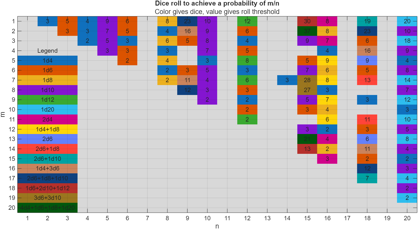
In the original xkcd, the situation described by the player has a probability of 2/9. Looking up the plot, row 2 column 9, shows that you need 16 or greater on (from the legend) 1d4+3d6, just as claimed.
If you missed the bit about convolutions, this is a super-neat trick
[v,c] = dicedist([4 6 6 6]);
bar(v,c)
% Probability distribution of dice given by d
function [vals,counts] = dicedist(d)
% d is a vector of number of sides
n = numel(d); % number of dice
% Use convolution to count the number of ways to get each roll value
counts = 1;
for k = 1:n
counts = conv(counts,ones(1,d(k)));
end
% Possible values range from n to sum(d)
maxtot = sum(d);
vals = n:maxtot;
end
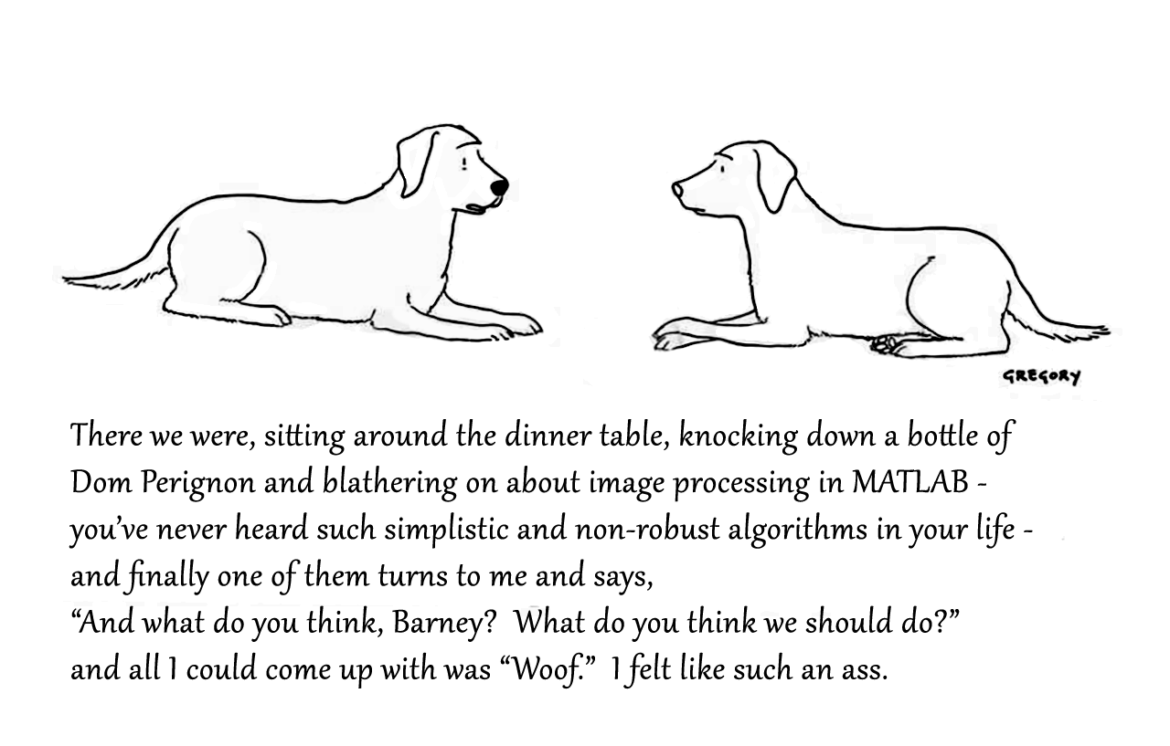
Attaching the Photoshop file if you want to modify the caption.
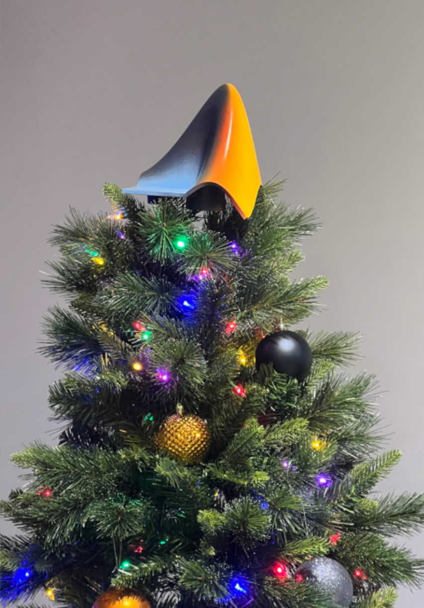
What better way to add a little holiday magic than the L-shaped membrane atop your evergreen? My colleagues output the shape and then added some thickness and an interior cylinder in Blender. Then, the shape was exported to STL and 3D printed (in several pieces). Then glued, sanded, primed, sanded again and painted. If you like, the STL file is attached. Thank you to https://blogs.mathworks.com/community/2013/06/20/paul-prints-the-l-shaped-membrane/ and a tip of the hat to MATLAB Ornament. Happy Holidays!


If you have a folder with an enormous number of files and want to use the uigetfile function to select specific files, you may have noticed a significant delay in displaying the file list.
Thanks to the assistance from MathWorks support, an interesting behavior was observed.
For example, if a folder such as Z:\Folder1\Folder2\data contains approximately 2 million files, and you attempt to use uigetfile to access files with a specific extension (e.g., *.ext), the following behavior occurs:
Method 1: This takes minutes to show me the list of all files
[FileName, PathName] = uigetfile('Z:\Folder1\Folder2\data\*.ext', 'File selection');
Method 2: This takes less than a second to display all files.
[FileName, PathName] = uigetfile('*.ext', 'File selection','Z:\Folder1\Folder2\data');
Method 3: This method also takes minutes to display the file list. What is intertesting is that this method is the same as Method 2, except that a file seperator "\" is added at the end of the folder string.
[FileName, PathName] = uigetfile('*.ext', 'File selection','Z:\Folder1\Folder2\data\');
I was informed that the Mathworks development team has been informed of this strange behaviour.
I am using 2023a, but think this should be the same for newer versions.
This post is more of a "tips and tricks" guide than a question.
If you have a folder with an enormous number of files and want to use the uigetfile function to select specific files, you may have noticed a significant delay in displaying the file list.
Thanks to the assistance from MathWorks support, an interesting behavior was observed.
For example, if a folder such as Z:\Folder1\Folder2\data contains approximately 2 million files, and you attempt to use uigetfile to access files with a specific extension (e.g., *.ext), the following behavior occurs:
Method 1: This takes minutes to show me the list of all files
[FileName, PathName] = uigetfile('Z:\Folder1\Folder2\data\*.ext', 'File selection');
Method 2: This takes less than a second to display all files.
[FileName, PathName] = uigetfile('*.ext', 'File selection','Z:\Folder1\Folder2\data');
Method 3: This method also takes minutes to display the file list. What is intertesting is that this method is the same as Method 2, except that a file seperator "\" is added at the end of the folder string.
[FileName, PathName] = uigetfile('*.ext', 'File selection','Z:\Folder1\Folder2\data\');
I was informed that the Mathworks development team has been informed of this strange behaviour.
I am using 2023a, but think this should be the same for newer versions.


Christmas is coming, here are two dynamic Christmas tree drawing codes:
Crystal XMas Tree
function XmasTree2024_1
fig = figure('Units','normalized', 'Position',[.1,.1,.5,.8],...
'Color',[0,9,33]/255, 'UserData',40 + [60,65,75,72,0,59,64,57,74,0,63,59,57,0,1,6,45,75,61,74,28,57,76,57,1,1]);
axes('Parent',fig, 'Position',[0,-1/6,1,1+1/3], 'UserData',97 + [18,11,0,13,3,0,17,4,17],...
'XLim',[-1.5,1.5], 'YLim',[-1.5,1.5], 'ZLim',[-.2,3.8], 'DataAspectRatio', [1,1,1], 'NextPlot','add',...
'Projection','perspective', 'Color',[0,9,33]/255, 'XColor','none', 'YColor','none', 'ZColor','none')
%% Draw Christmas tree
F = [1,3,4;1,4,5;1,5,6;1,6,3;...
2,3,4;2,4,5;2,5,6;2,6,3];
dP = @(V) patch('Faces',F, 'Vertices',V, 'FaceColor',[0 71 177]./255,...
'FaceAlpha',rand(1).*0.2+0.1, 'EdgeColor',[0 71 177]./255.*0.8,...
'EdgeAlpha',0.6, 'LineWidth',0.5, 'EdgeLighting','gouraud', 'SpecularStrength',0.3);
r = .1; h = .8;
V0 = [0,0,0; 0,0,1; 0,r,h; r,0,h; 0,-r,h; -r,0,h];
% Rotation matrix
Rx = @(V, theta) V*[1 0 0; 0 cos(theta) sin(theta); 0 -sin(theta) cos(theta)];
Rz = @(V, theta) V*[cos(theta) sin(theta) 0;-sin(theta) cos(theta) 0; 0 0 1];
N = 180; Vn = zeros(N, 3); eval(char(fig.UserData))
for i = 1:N
tV = Rz(Rx(V0.*(1.2 - .8.*i./N + rand(1).*.1./i^(1/5)), pi/3.*(1 - .6.*i./N)), i.*pi/8.1 + .001.*i.^2) + [0,0,.016.*i];
dP(tV); Vn(i,:) = tV(2,:);
end
scatter3(Vn(:,1).*1.02,Vn(:,2).*1.02,Vn(:,3).*1.01, 30, 'w', 'Marker','*', 'MarkerEdgeAlpha',.5)
%% Draw Star of Bethlehem
w = .3; R = .62; r = .4; T = (1/8:1/8:(2 - 1/8)).'.*pi;
V8 = [ 0, 0, w; 0, 0,-w;
1, 0, 0; 0, 1, 0; -1, 0, 0; 0,-1,0;
R, R, 0; -R, R, 0; -R,-R, 0; R,-R,0;
cos(T).*r, sin(T).*r, T.*0];
F8 = [1,3,25; 1,3,11; 2,3,25; 2,3,11; 1,7,11; 1,7,13; 2,7,11; 2,7,13;
1,4,13; 1,4,15; 2,4,13; 2,4,15; 1,8,15; 1,8,17; 2,8,15; 2,8,17;
1,5,17; 1,5,19; 2,5,17; 2,5,19; 1,9,19; 1,9,21; 2,9,19; 2,9,21;
1,6,21; 1,6,23; 2,6,21; 2,6,23; 1,10,23; 1,10,25; 2,10,23; 2,10,25];
V8 = Rx(V8.*.3, pi/2) + [0,0,3.5];
patch('Faces',F8, 'Vertices',V8, 'FaceColor',[255,223,153]./255,...
'EdgeColor',[255,223,153]./255, 'FaceAlpha', .2)
%% Draw snow
sXYZ = rand(200,3).*[4,4,5] - [2,2,0];
sHdl1 = plot3(sXYZ(1:90,1),sXYZ(1:90,2),sXYZ(1:90,3), '*', 'Color',[.8,.8,.8]);
sHdl2 = plot3(sXYZ(91:200,1),sXYZ(91:200,2),sXYZ(91:200,3), '.', 'Color',[.6,.6,.6]);
annotation(fig,'textbox',[0,.05,1,.09], 'Color',[1 1 1], 'String','Merry Christmas Matlaber',...
'HorizontalAlignment','center', 'FontWeight','bold', 'FontSize',48,...
'FontName','Times New Roman', 'FontAngle','italic', 'FitBoxToText','off','EdgeColor','none');
% Rotate the Christmas tree and let the snow fall
for i=1:1e8
sXYZ(:,3) = sXYZ(:,3) - [.05.*ones(90,1); .06.*ones(110,1)];
sXYZ(sXYZ(:,3)<0, 3) = sXYZ(sXYZ(:,3) < 0, 3) + 5;
sHdl1.ZData = sXYZ(1:90,3); sHdl2.ZData = sXYZ(91:200,3);
view([i,30]); drawnow; pause(.05)
end
end

Curved XMas Tree
function XmasTree2024_2
fig = figure('Units','normalized', 'Position',[.1,.1,.5,.8],...
'Color',[0,9,33]/255, 'UserData',40 + [60,65,75,72,0,59,64,57,74,0,63,59,57,0,1,6,45,75,61,74,28,57,76,57,1,1]);
axes('Parent',fig, 'Position',[0,-1/6,1,1+1/3], 'UserData',97 + [18,11,0,13,3,0,17,4,17],...
'XLim',[-6,6], 'YLim',[-6,6], 'ZLim',[-16, 1], 'DataAspectRatio', [1,1,1], 'NextPlot','add',...
'Projection','perspective', 'Color',[0,9,33]/255, 'XColor','none', 'YColor','none', 'ZColor','none')
%% Draw Christmas tree
[X,T] = meshgrid(.4:.1:1, 0:pi/50:2*pi);
XM = 1 + sin(8.*T).*.05;
X = X.*XM; R = X.^(3).*(.5 + sin(8.*T).*.02);
dF = @(R, T, X) surf(R.*cos(T), R.*sin(T), -X, 'EdgeColor',[20,107,58]./255,...
'FaceColor', [20,107,58]./255, 'FaceAlpha',.2, 'LineWidth',1);
CList = [254,103,110; 255,191,115; 57,120,164]./255;
for i = 1:5
tR = R.*(2 + i); tT = T+i; tX = X.*(2 + i) + i;
SFHdl = dF(tR, tT, tX);
[~, ind] = sort(SFHdl.ZData(:)); ind = ind(1:8);
C = CList(randi([1,size(CList,1)], [8,1]), :);
scatter3(tR(ind).*cos(tT(ind)), tR(ind).*sin(tT(ind)), -tX(ind), 120, 'filled',...
'CData', C, 'MarkerEdgeColor','none', 'MarkerFaceAlpha',.3)
scatter3(tR(ind).*cos(tT(ind)), tR(ind).*sin(tT(ind)), -tX(ind), 60, 'filled', 'CData', C)
end
%% Draw Star of Bethlehem
Rx = @(V, theta) V*[1 0 0; 0 cos(theta) sin(theta); 0 -sin(theta) cos(theta)];
% Rz = @(V, theta) V*[cos(theta) sin(theta) 0;-sin(theta) cos(theta) 0; 0 0 1];
w = .3; R = .62; r = .4; T = (1/8:1/8:(2 - 1/8)).'.*pi;
V8 = [ 0, 0, w; 0, 0,-w;
1, 0, 0; 0, 1, 0; -1, 0, 0; 0,-1,0;
R, R, 0; -R, R, 0; -R,-R, 0; R,-R,0;
cos(T).*r, sin(T).*r, T.*0];
F8 = [1,3,25; 1,3,11; 2,3,25; 2,3,11; 1,7,11; 1,7,13; 2,7,11; 2,7,13;
1,4,13; 1,4,15; 2,4,13; 2,4,15; 1,8,15; 1,8,17; 2,8,15; 2,8,17;
1,5,17; 1,5,19; 2,5,17; 2,5,19; 1,9,19; 1,9,21; 2,9,19; 2,9,21;
1,6,21; 1,6,23; 2,6,21; 2,6,23; 1,10,23; 1,10,25; 2,10,23; 2,10,25];
V8 = Rx(V8.*.8, pi/2) + [0,0,-1.3];
patch('Faces',F8, 'Vertices',V8, 'FaceColor',[255,223,153]./255,...
'EdgeColor',[255,223,153]./255, 'FaceAlpha', .2)
annotation(fig,'textbox',[0,.05,1,.09], 'Color',[1 1 1], 'String','Merry Christmas Matlaber',...
'HorizontalAlignment','center', 'FontWeight','bold', 'FontSize',48,...
'FontName','Times New Roman', 'FontAngle','italic', 'FitBoxToText','off','EdgeColor','none');
%% Draw snow
sXYZ = rand(200,3).*[12,12,17] - [6,6,16];
sHdl1 = plot3(sXYZ(1:90,1),sXYZ(1:90,2),sXYZ(1:90,3), '*', 'Color',[.8,.8,.8]);
sHdl2 = plot3(sXYZ(91:200,1),sXYZ(91:200,2),sXYZ(91:200,3), '.', 'Color',[.6,.6,.6]);
for i=1:1e8
sXYZ(:,3) = sXYZ(:,3) - [.1.*ones(90,1); .12.*ones(110,1)];
sXYZ(sXYZ(:,3)<-16, 3) = sXYZ(sXYZ(:,3) < -16, 3) + 17.5;
sHdl1.ZData = sXYZ(1:90,3); sHdl2.ZData = sXYZ(91:200,3);
view([i,30]); drawnow; pause(.05)
end
end

I wish all MATLABers a Merry Christmas in advance!
Hi! My name is Mike McLernon, and I’m a product marketing engineer with MathWorks. In my role, I look at the trends ongoing in the wireless industry, across lots of different standards (think 5G, WLAN, SatCom, Bluetooth, etc.), and I seek to shape and guide the software that MathWorks builds to respond to these trends. That’s all about communicating within the Mathworks organization, but every so often it’s worth communicating these trends to our audience in the world at large. Many of the people reading this are engineers (or engineers at heart), and we all want to know what’s happening in the geek world around us. I think that now is one of these times to communicate an important milestone. So, without further ado . . .
Bluetooth 6.0 is here! Announced in September by the Bluetooth Special Interest Group (SIG), it’s making more advances in its quest to create a “world without wires”. A few of the salient features in Bluetooth 6.0 are:
- Channel sounding (for accurate distance measurements)
- Decision-based advertising filtering (for more efficient channel scanning)
- Monitoring advertisers (for improved energy efficiency when devices come into and go out of range)
- Frame space updates (for both higher throughput and better coexistence management)
Bluetooth 6.0 includes other features as well, but the SIG has put special promotional emphasis on channel sounding (CS), which once upon a time was called High Accuracy Distance Measurement (HADM). The SIG has said that CS is a step towards true distance awareness, and 10 cm ranging accuracy. I think their emphasis is in exactly the right place, so let’s learn more about this technology and how it is used.
CS can be used for the following use cases:
- Keyless vehicle entry, performed by communication between a key fob or phone and the car’s anchor points
- Smart locks, to permit access only when an authorized device is within a designated proximity to the locks
- Geofencing, to limit access to designated areas
- Warehouse management, to monitor inventory and manage logistics
- Asset tracking for virtually any object of interest

In the past, Bluetooth devices would use a received signal strength indicator (RSSI) measurement to infer the distance between two of them. They would assume a free space path loss on the link, and use a straightforward equation to estimate distance:


 where
whereSo in this method,  . But if the signal suffers more loss from multipath or shadowing, then the distance would be overestimated. Something better needed to be found.
 . But if the signal suffers more loss from multipath or shadowing, then the distance would be overestimated. Something better needed to be found.
Bluetooth 6.0 introduces not one, but two ways to accurately measure distance:
- Round-trip time (RTT) measurement
- Phase-based ranging (PBR) measurement
The RTT measurement method uses the fact that the Bluetooth signal time of flight (TOF) between two devices is half the RTT. It can then accurately compute the distance d as
 , where c is again the speed of light. This method requires accurate measurements of the time of departure (TOD) of the outbound signal from device 1 (the Initiator), time of arrival (TOA) of the outbound signal to device 2 (the Reflector), TOD of the return signal from device 2, and TOA of the return signal to device 1. The diagram below shows the signal paths and the times.
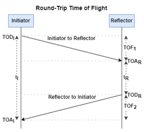
If you want to see how you can use MATLAB to simulate the RTT method, take a look at Estimate Distance Between Bluetooth LE Devices by Using Channel Sounding and Round-Trip Timing.
The PBR method uses two Bluetooth signals of different frequencies to measure distance. These signals are simply tones – sine waves. Without going through the derivation, PBR calculates distance d as
The mod() operation is needed to eliminate ambiguities in the distance calculation and the final division by two is to convert a round trip distance to a one-way distance. Because a given phase difference value can hold true for an infinite number of distance values, the mod() operation chooses the smallest distance that satisfies the equation. Also, these tones can be as close as 1 MHz apart. In that case, the maximum resolvable distance measurement is about 150 m. The plot below shows that ambiguity and repetition in distance measurement.
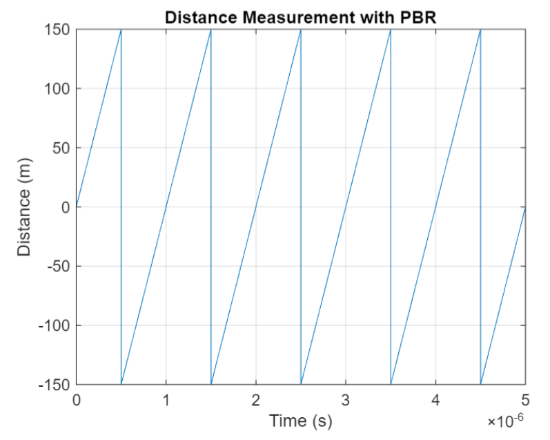
If you want to see how you can use MATLAB to simulate the PBR method, take a look at Estimate Distance Between Bluetooth LE Devices by Using Channel Sounding and Phase-Based Ranging.
Bluetooth 6.0 outlines RTT and PBR distance measurement methods, but CS does not mandate a specific algorithm for calculating distance estimates. This flexibility allows device manufacturers to tailor solutions to various use cases, balancing computational complexity with required accuracy and adapting to different radio environments. Examples include simple phase difference calculations and FFT-based methods.
Although Bluetooth 6.0 is now out, it is far from a finished version. The SIG is actively working through the ratification process for two major extensions:
- High Data Throughput, up to 8 Mbps
- 5 and 6 GHz operation
See the last few minutes of this video from the SIG to learn more about these exciting future developments. And if you want to see more Bluetooth blogs, give a review of this one! Finally, if you have specific Bluetooth questions, give me a shout and let’s start a discussion!
Christmas season is underway at my house:

(Sorry - the ornament is not available at the MathWorks Merch Shop -- I made it with a 3-D printer.)
So I made this.
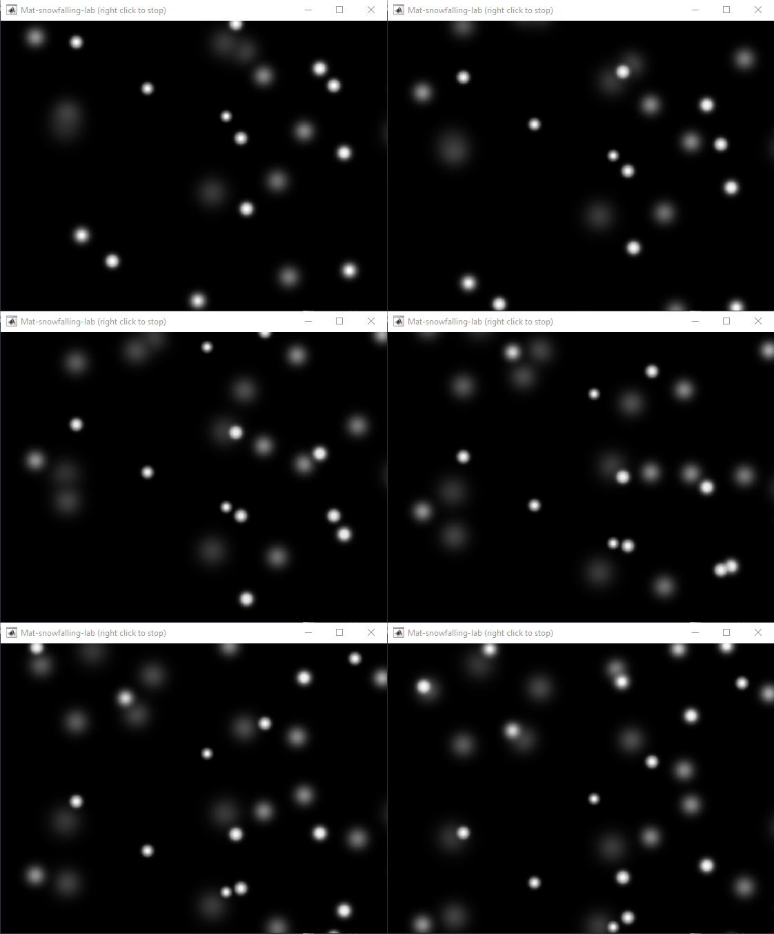
clear
close all
clc
% inspired from: https://www.youtube.com/watch?v=3CuUmy7jX6k
%% user parameters
h = 768;
w = 1024;
N_snowflakes = 50;
%% set figure window
figure(NumberTitle="off", ...
name='Mat-snowfalling-lab (right click to stop)', ...
MenuBar="none")
ax = gca;
ax.XAxisLocation = 'origin';
ax.YAxisLocation = 'origin';
axis equal
axis([0, w, 0, h])
ax.Color = 'k';
ax.XAxis.Visible = 'off';
ax.YAxis.Visible = 'off';
ax.Position = [0, 0, 1, 1];
%% first snowflake
ht = gobjects(1, 1);
for i=1:length(ht)
ht(i) = hgtransform();
ht(i).UserData = snowflake_factory(h, w);
ht(i).Matrix(2, 4) = ht(i).UserData.y;
ht(i).Matrix(1, 4) = ht(i).UserData.x;
im = imagesc(ht(i), ht(i).UserData.img);
im.AlphaData = ht(i).UserData.alpha;
colormap gray
end
%% falling snowflake
tic;
while true
% add a snowflake every 0.3 seconds
if toc > 0.3
if length(ht) < N_snowflakes
ht = [ht; hgtransform()];
ht(end).UserData = snowflake_factory(h, w);
ht(end).Matrix(2, 4) = ht(end).UserData.y;
ht(end).Matrix(1, 4) = ht(end).UserData.x;
im = imagesc(ht(end), ht(end).UserData.img);
im.AlphaData = ht(end).UserData.alpha;
colormap gray
end
tic;
end
ax.CLim = [0, 0.0005]; % prevent from auto clim
% move snowflakes
for i = 1:length(ht)
ht(i).Matrix(2, 4) = ht(i).Matrix(2, 4) + ht(i).UserData.velocity;
end
if strcmp(get(gcf, 'SelectionType'), 'alt')
set(gcf, 'SelectionType', 'normal')
break
end
drawnow
% delete the snowflakes outside the window
for i = length(ht):-1:1
if ht(i).Matrix(2, 4) < -length(ht(i).Children.CData)
delete(ht(i))
ht(i) = [];
end
end
end
%% snowflake factory
function snowflake = snowflake_factory(h, w)
radius = round(rand*h/3 + 10);
sigma = radius/6;
snowflake.velocity = -rand*0.5 - 0.1;
snowflake.x = rand*w;
snowflake.y = h - radius/3;
snowflake.img = fspecial('gaussian', [radius, radius], sigma);
snowflake.alpha = snowflake.img/max(max(snowflake.img));
end
We are thrilled to announce the grand prize winners of our MATLAB Shorts Mini Hack contest! This year, we invited the MATLAB Graphics and Charting team, the authors of the MATLAB functions used in every entry, to be our judges. After careful consideration, they have selected the top three winners:
Judge comments: Realism & detailed comments; wowed us with Manta Ray
2nd place – Jenny Bosten
Judge comments: Topical hacks : Auroras & Wind turbine; beautiful landscapes & nightscapes
3rd place - Vasilis Bellos
Judge comments: Nice algorithms & extra comments; can’t go wrong with Pumpkins
Judge comments: Impressive spring & cubes!
In addition, after validating the votes, we are pleased to announce the top 10 participants on the leaderboard:
Congratulations to all! Your creativity and skills have inspired many of us to explore and learn new skills, and make this contest a big success!
Dear MATLAB contest enthusiasts,
Welcome to the third installment of our interview series with top contest participants! This time we had the pleasure of talking to our all-time rock star – @Jenny Bosten. Every one of her entries is a masterpiece, demonstrating a deep understanding of the relationship between mathematics and aesthetics. Even Cleve Moler, the original author of MATLAB, is impressed and wrote in his blog: "Her code for Time Lapse of Lake View to the West shows she is also a wizard of coordinate systems and color maps."
you to read it to learn more about Jenny’s journey, her creative process, and her favorite entries.
Question: Who would you like to see featured in our next interview? Let us know your thoughts in the comments!
Over the past 4 weeks, 250+ creative short movies have been crafted. We had a lot of fun and, more importantly, learned new skills from each other! Now it’s time to announce week 4 winners.
Nature:
3D:
Seamless loop:
Holiday:
Fractal:
Congratulations! Each of you won your choice of a T-shirt, a hat, or a coffee mug. We will contact you after the contest ends.
Weekly Special Prizes
Thank you for sharing your tips & tricks with the community. These great technical articles will benefit community users for many years. You won a limited-edition pair of MATLAB Shorts!

In week 5, let’s take a moment to sit back, explore all of the interesting entries, and cast your votes. Reflect what you have learned or which entries you like most. Share anything in our Discussions area! There is still time to win our limited-edition MATLAB Shorts.
Hi everyone, I wrote several fancy functions that may help your coding experience, since they are in very early developing stage, I will be thankful if anyone could try them and give some feedbacks. Currently I have following:
- fstr: a Python f-string like expression
- printf: an easy to use fprintf function, accepts multiple arguments with seperator, end string control.
I will bring more functions or packages like logger when I am available.
The code is open sourced at GitHub with simple examples: https://github.com/bentrainer/MMGA


