Generalized Predictive Control (a type of MPC)
Versione 1.0.1 (335 KB) da
Alireza Esmailnezhad
This project lets you to design a Generalized Predictive Controller (GPC) for MIMO systems, includes any number of inputs k and outputs p
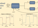
GPC, a type of Model Predictive Controller (MPC), was introduced by David W. Clarke in 1987. In this code, I have implemented the GPC algorithm to design a predictive controller for a given transfer function system. The code is highly versatile, allowing users to define any number of inputs and outputs (subsystems). The algorithm automatically designs a predictive controller for all subsystems. While this version of GPC performs well for stable systems, SGPC or CRHPC controllers are recommended for unstable systems. These will be provided in future versions. The block diagram of a model predictive control is shown as below :

In the figure above:
- N represents the model horizon.
- M is the control horizon.
- P is the prediction horizon.
It's worth noting that GPC does not have a model horizon because it uses a transfer function model, unlike other MPC algorithms. Instead, it constructs the cost function by solving the Diophantine equation (Bezout identity).
R and Q are the matrix weights of the cost function.
Parameters and Inputs:
- Define Inputs and Outputs: First, the user must define the number of inputs and outputs of the process.
- Subsystems: Subsystems of the MIMO system should be defined as transfer functions, as shown in the code example.
- Simulation Settings: Choose an appropriate sample time and set the start and end times for the simulation (in seconds).
- Horizon Selection: Select the prediction and control horizons.
- Cost Function Weights: Choose suitable cost function weights.
- Reference Signal Smoothing: Optionally, use a smoothing filter for the reference signal (desired output) by setting its pole placement arbitrarily.
- Design Method: Decide whether the GPC design will be programmed or unprogrammed.
- Programmed Method: Predictive (future) references are known.
- Unprogrammed Method: Predictive (future) references are unknown, so set all future references the same as the current reference signal value.
- Reference Signal: By default, the reference signal is set to square and sine waves. Users can select one or define their own desired reference signal. Additionally, users can set the reference signal period, time-shifts in different channels, and the desired amplitude for each channel individually.
- Disturbance Settings: Optionally, set disturbances for the controlled signal.
- Noise Settings: Optionally, set output noise levels.
Simulation Results:
After the simulation, results are displayed in a figure containing: a) A comparison of each process output channel with the corresponding reference signal. b) A comparison of each process output channel with the corresponding model output channel. c) Values and derivatives of each control signal channel. d) Disturbances and noise for their corresponding channels.
This code's flexibility allows users to modify various parameters and settings to suit their specific needs, making it a powerful tool for designing predictive controllers.
Example results for a single input & single output system:

Example results for a 2 inputs & 2 outputs system:

Reference :
Clarke, D. W., Mohtadi, C., & Tuffs, P. S. (1987). Generalized predictive control—Part I. The basic algorithm. Automatica, 23(2), 137-148.
Cita come
Alireza Esmailnezhad (2025). Generalized Predictive Control (a type of MPC) (https://it.mathworks.com/matlabcentral/fileexchange/169131-generalized-predictive-control-a-type-of-mpc), MATLAB Central File Exchange. Recuperato .
Compatibilità della release di MATLAB
Creato con
R2022a
Compatibile con qualsiasi release
Compatibilità della piattaforma
Windows macOS LinuxTag
Community Treasure Hunt
Find the treasures in MATLAB Central and discover how the community can help you!
Start Hunting!Scopri Live Editor
Crea script con codice, output e testo formattato in un unico documento eseguibile.
| Versione | Pubblicato | Note della release | |
|---|---|---|---|
| 1.0.1 | change in title and description |
|
|
| 1.0.0 |
|

