Modeling Custom Satellite Attitude and Gimbal Steering

This example shows how to point a satellite or gimbal in a satellite scenario using logged orientation data from a timetable or timeseries. It uses data generated by the Aerospace Blockset™ Spacecraft Dynamics block. For more information about the data and how to generate it, see the Aerospace Blockset example Analyzing Spacecraft Attitude Profiles with Satellite Scenario.

The satelliteScenario object lets you load previously generated, time-stamped ephemeris and attitude data into a scenario as timeseries or timetable objects. Data is interpolated in the scenario object to align with the scenario time steps, allowing you to incorporate data generated in a Simulink model into either a new or existing satelliteScenario object. For this example, the satellite orbit and attitude states are precomputed by the Spacecraft Dynamics block. Load this data to the workspace and use it to model a satellite to a satelliteScenario object for access analysis.

Define Mission Parameters and Satellite Initial Conditions

Specify a start date and duration for the mission. This example uses MATLAB® structures to organize mission data. These structures make accessing data later in the example more intuitive. They also help declutter the global base workspace.

mission.StartDate = datetime(2021,1,1,12,0,0);
mission.Duration = hours(1.5);

Specify initial orbital elements for the satellite.

mission.Satellite.SemiMajorAxis  = 7.2e6; % meters
mission.Satellite.Eccentricity   = .05;
mission.Satellite.Inclination    = 70;    % deg
mission.Satellite.ArgOfPeriapsis = 0;     % deg
mission.Satellite.RAAN           = 215;   % deg
mission.Satellite.TrueAnomaly    = 200;   % deg

Specify an initial attitude state for the satellite.

mission.Satellite.q0 = [1, 0, 0, 0];
mission.Satellite.pqr = [0, 0, 0]; % deg/s

Load Ephemeris and Attitude Profile

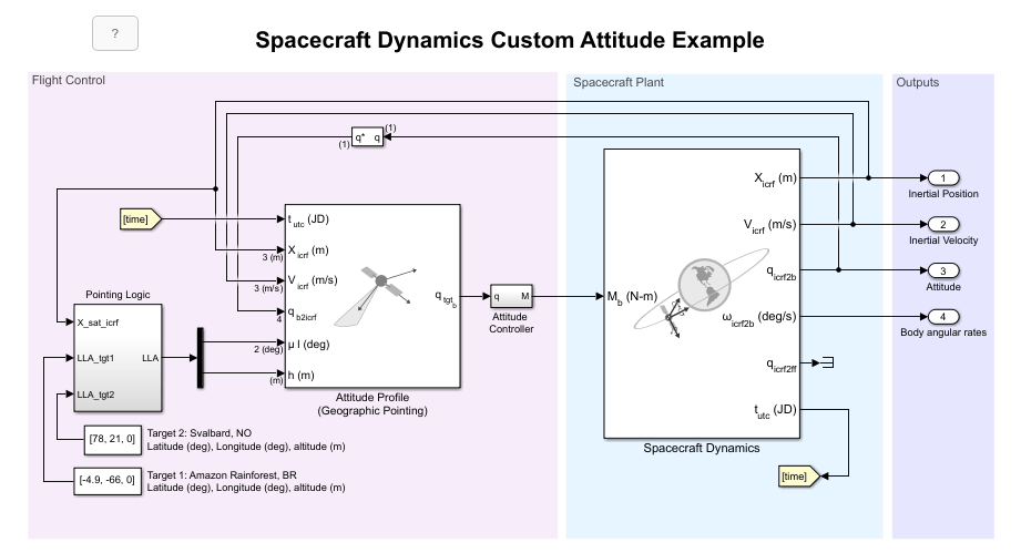
The Simulink® model used to generate data for this example is configured to perform an Earth Observation mission during which a satellite performs a flyover of a region of the Amazon Rainforest to capture images of, and track deforestation trends in, the area.

The satellite points at the nadir when not actively imaging or downlinking to the ground station in Svalbard, NO. The Aerospace Blockset Attitude Profile block calculates commanded attitude. The satellite uses spherical harmonic gravity model EGM2008 for orbit propagation. Gravity gradient torque contributions are also included in attitude dynamics. For more information about this model, see the Aerospace Blockset example Analyzing Spacecraft Attitude Profiles with Satellite Scenario.

The timetable objects contain position and attitude data for the satellite throughout the mission. The data is referenced in the inertial (ICRF/GCRF) reference frame. Attitude values are expressed as quaternions, although Euler angles are also supported.

mission.Data = load("SatelliteScenarioCustomAttitudeData.mat", "PositionTimeTableGCRF", "AttitudeTimeTableGCRF2Body");
display(mission.Data.PositionTimeTableGCRF)

  1148×1 timetable

       Time                         Data                  
    __________    ________________________________________

    0 sec         5.2953e+06      4.784e+06     -2.422e+06
    5 sec         5.2783e+06     4.7859e+06    -2.4532e+06
    10 sec        5.2611e+06     4.7877e+06    -2.4842e+06
    13.263 sec    5.2499e+06     4.7888e+06    -2.5045e+06
    15 sec        5.2439e+06     4.7894e+06    -2.5152e+06

        :                            :                    

    5380 sec      6.3454e+06     3.4735e+06     2.1279e+06
    5385 sec      6.3479e+06     3.4893e+06     2.0962e+06
    5390 sec      6.3503e+06     3.5051e+06     2.0645e+06
    5395 sec      6.3526e+06     3.5207e+06     2.0327e+06
    5400 sec      6.3547e+06     3.5363e+06     2.0009e+06

	Display all 1148 rows.

display(mission.Data.AttitudeTimeTableGCRF2Body)

  1148×1 timetable

       Time                             Data                      
    __________    ________________________________________________

    0 sec            0.1509      0.48681      0.30311     -0.80522
    5 sec           0.15061      0.48761       0.3033     -0.80472
    10 sec          0.15003      0.48914      0.30368     -0.80375
    13.263 sec      0.14977      0.48986      0.30387     -0.80329
    15 sec          0.14967      0.49013      0.30395     -0.80311

        :                                :                        

    5380 sec      -0.043839     -0.72806     -0.33468      0.59666
    5385 sec       -0.04461     -0.72663      -0.3346      0.59838
    5390 sec       -0.04538     -0.72521     -0.33451      0.60009
    5395 sec      -0.046149     -0.72378     -0.33443      0.60181
    5400 sec      -0.046919     -0.72235     -0.33434      0.60351

	Display all 1148 rows.

Create the Satellite Scenario

Create a satellite scenario object to use for analysis. Specify a timestep of 1 minute.

scenario = satelliteScenario(mission.StartDate, ...
    mission.StartDate + mission.Duration, 60);

Add the two targets as ground stations in Brazil and Svalbard.

gsNO = groundStation(scenario, 78, 21, Name="Svalbard, NO")

gsNO = 
  GroundStation with properties:

                 Name:  Svalbard, NO
                   ID:  1
             Latitude:  78 degrees
            Longitude:  21 degrees
             Altitude:  0 meters
    MinElevationAngle:  0 degrees
       ConicalSensors:  [1x0 matlabshared.satellitescenario.ConicalSensor]
              Gimbals:  [1x0 matlabshared.satellitescenario.Gimbal]
         Transmitters:  [1x0 satcom.satellitescenario.Transmitter]
            Receivers:  [1x0 satcom.satellitescenario.Receiver]
             Accesses:  [1x0 matlabshared.satellitescenario.Access]
          MarkerColor:  [1 0.4118 0.1608]
           MarkerSize:  6
            ShowLabel:  true
       LabelFontColor:  [1 1 1]
        LabelFontSize:  15

gsAmazon = groundStation(scenario, -4.9, -66, Name="Amazon Rainforest")

gsAmazon = 
  GroundStation with properties:

                 Name:  Amazon Rainforest
                   ID:  2
             Latitude:  -4.9 degrees
            Longitude:  -66 degrees
             Altitude:  0 meters
    MinElevationAngle:  0 degrees
       ConicalSensors:  [1x0 matlabshared.satellitescenario.ConicalSensor]
              Gimbals:  [1x0 matlabshared.satellitescenario.Gimbal]
         Transmitters:  [1x0 satcom.satellitescenario.Transmitter]
            Receivers:  [1x0 satcom.satellitescenario.Receiver]
             Accesses:  [1x0 matlabshared.satellitescenario.Access]
          MarkerColor:  [1 0.4118 0.1608]
           MarkerSize:  6
            ShowLabel:  true
       LabelFontColor:  [1 1 1]
        LabelFontSize:  15

Add the Satellite From the Loaded Trajectory

Add the observation satellite to the scenario.

sat = satellite(scenario, mission.Data.PositionTimeTableGCRF, ...
    "CoordinateFrame", "inertial", "Name", "ObservationSat");

Add a conical sensor to the satellite, with a 35 deg half angle to represent the onboard camera. Enable field of view visualization in the scenario viewer. To assist in visualization, the sensor is mounted 10m from the satellite in the +z direction.

snsr = conicalSensor(sat, MaxViewAngle=70, MountingLocation=[0 0 10]);
fieldOfView(snsr);

Add access between the conical sensor and the two ground stations.

acNO = access(snsr, gsNO)

acNO = 
  Access with properties:

    Sequence:  [4 1]
    LineWidth:  3
    LineColor:  [0.3922 0.8314 0.0745]

acAmazon = access(snsr, gsAmazon)

acAmazon = 
  Access with properties:

    Sequence:  [4 2]
    LineWidth:  3
    LineColor:  [0.3922 0.8314 0.0745]

Point the Satellite With the Loaded Attitude Profile

Use the pointAt method to associate the logged attitude timetable with the satellite. Parameter ExtrapolationMethod controls the pointing behavior outside of the timetable range.

pointAt(sat, mission.Data.AttitudeTimeTableGCRF2Body, ...
    "CoordinateFrame", "inertial", "Format", "quaternion", "ExtrapolationMethod", "nadir");

Visualize the Scenario

Open the Satellite Scenario Viewer to view and interact with the scenario.

viewer1 = satelliteScenarioViewer(scenario);

The satellite points at the nadir to begin the scenario. As it nears Target 1 in the Amazon Rainforest, it slews to point and track this target.

After the imaging segment is complete, the satellite returns to pointing at the nadir.

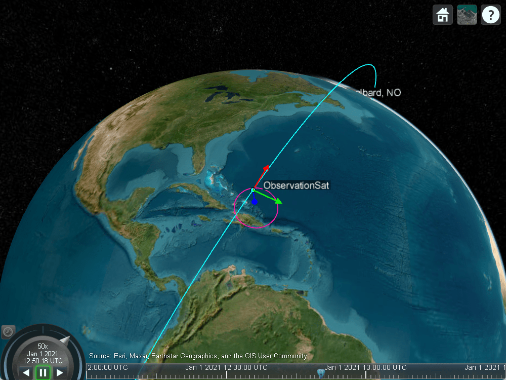
As the satellite comes into range of the arctic ground station, it slews to point at this target.

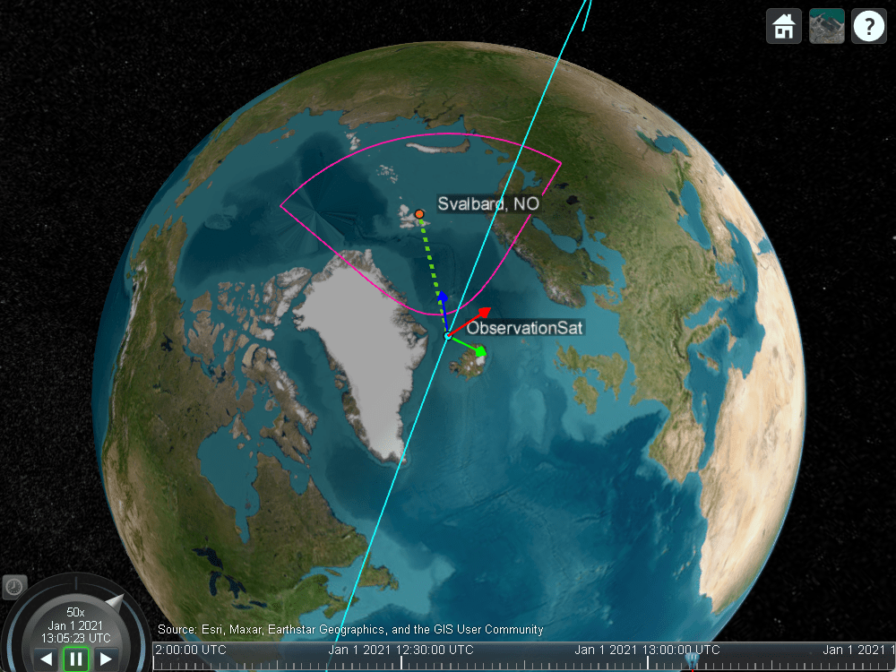
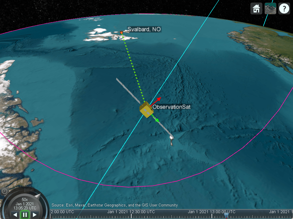
Custom Gimbal Steering

This example shows how to import custom attitude data for a simple Earth Observation satellite mission, where the onboard camera is fixed to the satellite body. Another common approach is to fix the sensor on a gimbal and orient the sensor by manuevering the gimbal, rather than the spacecraft body itself. Modify the above scenario to mount the sensor on a gimbal and steer the gimbal to perform uniform sweeps of the area directly below the satellite.

Reset the satellite to always point at the nadir, overwriting the previously provided custom attitude profile.

delete(viewer1);
pointAt(sat, "nadir");

Delete the existing sensor object to remove it from the satellite and attach a new sensor with the same properties to a gimbal.

delete(snsr);
gim = gimbal(sat);
snsr = conicalSensor(gim, MaxViewAngle=70, MountingLocation=[0 0 10]);
fieldOfView(snsr);

Define azimuth and elevation angles for gimbal steering to model a sweeping pattern over time below the satellite.

gimbalSweep.Time = seconds(1:50:5000)';

gimbalSweep.Az = [...
    45*ones(1,7),...
    45:-5:-45,...
    -45*ones(1,13),...
    -45:5:45,...
    45*ones(1,13),...
    45:-5:-45,...
    -45*ones(1,13)];
gimbalSweep.Az(end-2:end) = [];
gimbalSweep.Az = gimbalSweep.Az + 90;

gimbalSweep.El = [...
    0:-5:-30,...
    -30*ones(1,19),...
    -30:5:30,...
    30*ones(1,19),...
    30:-5:-30,...
    -30*ones(1,19),...
    -30:5:30];
gimbalSweep.El(end-2:end) = [];

Plot the commanded azimuth and elevation values over time.

figure(1)
hold on;
plot(gimbalSweep.Time', gimbalSweep.Az);
plot(gimbalSweep.Time', gimbalSweep.El);
hold off;
legend(["Az (deg)", "El (deg)"]);

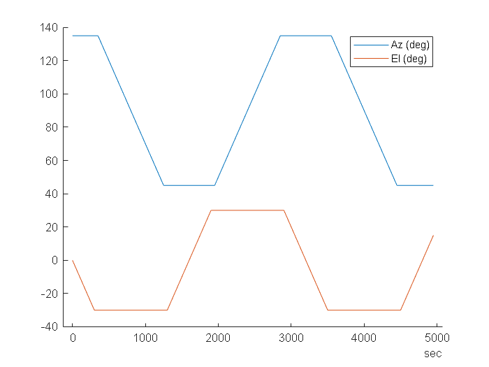
Store the azimuth and elevation angles in a timetable.

gimbalSweep.TT = timetable(gimbalSweep.Time, [gimbalSweep.Az', gimbalSweep.El']);

Steer the gimbal with the timetable. The gimbal returns to its default orientation for timesteps that are outside of the provided data.

pointAt(gim, gimbalSweep.TT);

View the updated scenario in the Satellite Scenario Viewer.

viewer2 = satelliteScenarioViewer(scenario);