Field Calculation in Antennas

Field Calculation in Metal Antennas

The electromagnetic analysis of an antenna or array starts from determining its equivalent current density. You can compute the current density using the field boundary conditions on the antenna’s surface or volume.

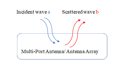
Incident excitation field E_i induces equivalent current J to produce scattered fields E_s and H_s.

Use the method-of-moments (MoM) technique described in Method of Moments Solver for Metal Structures to calculate the equivalent current density for metal only antennas. For the MoM technique, you can express the total current density as a weighted linear combination of N number basis functions (f_n^M) as

$$J={\displaystyle \sum _{n=1}^N{I}_n{f}_n^M}$$

Where the weighting coefficient of the n^th basis function is I_n. After calculating the current the current density vector J, compute the scattered electric (E_s) and magnetic (H_s) fields

$$E_s=E_s^M=\frac{-j\omega {\mu }_0}{4\pi }{\displaystyle \sum _{n=1}^{N_M}{I}_n}{\displaystyle \underset{S}{\overset{}{\int }}{f}_n^M}(r^{\text{'}})G(r,r^{\text{'}})d{s}^{\text{'}}-\frac{1}{4\pi \omega {\epsilon }_0}{\displaystyle \sum _{n=1}^{N_M}{I}_n}{\displaystyle \underset{S}{\overset{}{\int }}\nabla f_n^M}(r^{\text{'}}){\nabla }_{r}G(r,r^{\text{'}})ds$$

The curl of the magnetic vector potential gives the scattered magnetic field of the metal antenna

$$H_s=H_s^M=-\frac{1}{4\pi }{\displaystyle \sum _{n=1}^{N_M}{I}_n}{\displaystyle \underset{S}{\overset{\infty }{\int }}{f}_n^M}(r^{\text{'}})\times {\nabla }_{r}G(r,r^{\text{'}})ds$$

where the location of the source current density is r' and the observation location is r. The free-space Green’s function is

$$G(r,r^{\text{'}})=\frac{e^{-jk\left|r-r^{\text{'}}\right|}}{\left|r-r^{\text{'}}\right|}$$

where the free-space propagation constant is k. The observation location can be either in the near field region or in the far-field region with respect to the source current location. For a certain observation location $$r=[r_x{r}_y{r}_z]$$ each of the electric field E_s^M and magnetic field H_s^M is a 3-by-1 vector with components along three orthogonal co-ordinate axes. If the observation location is in the far-field region, the radial components of the electric and magnetic fields are negligible.

Field Calculation in Metal-Dielectric Antenna

For a metal-dielectric antenna, the total scattered electric and magnetic fields are a superposition of the fields ,(E_s^M,H_s^M) due to the metal surface current and the fields (E_s^DH_s^D) due to volume polarization current of the dielectric. In Method of Moments Solver for Metal and Dielectric Structures, the fields due to the dielectric current are given by:

$$E_s^D=\frac{{\omega }^2{\mu }_0}{4\pi }{\displaystyle \sum _{n=1}^{N_T}{D}_n{\displaystyle \sum _{p=1}^P{K}_p}}{\displaystyle \underset{V_p}{\int }G(r,r^{\text{'}})f_{np}}(r^{\text{'}})d{r}^{\text{'}}-\frac{1}{4\pi {\epsilon }_0}{\displaystyle \sum _{n=1}^{N_T}{D}_n{\displaystyle \sum _{q=1}^Q{\widehat{K}}_q{\displaystyle \underset{{\Omega }_q}{\int }{\nabla }_r}}}G(r,r^{\text{'}})f$$

$$H_s^D=-\frac{j\omega }{4\pi }{\displaystyle \sum _{n=1}^{N_T}{D}_n{\displaystyle \sum _{p=1}^P{K}_p}}{\displaystyle \underset{V_p}{\int }(f_{np}}(r^{\text{'}})\times {\nabla }_{r}G(r,r^{\text{'}}))d{r}^{\text{'}}$$

So the total scattered field from metal to dielectric is:

$$\begin{array}{l}{E}_s^{}=E_s^M+E_s^D\\ H_s^{}=H_s^M+H_s^D\end{array}$$

Field Parameters

The electric and magnetic fields at a near or far-field location is determined using the EHfields function.

Directivity

Radiation intensity of the antenna for a far-field sphere of radius R is

$$U(\theta ,\varphi )=\frac{R}{2{\eta }_0}{\left|E_s(R,\theta ,\varphi )\right|}^2$$

By default, R = 100λ is considered in Antenna Toolbox™ for pattern calculation. The free-space wavelength at minimum frequency is λ.

For a far-field location, the default electric field is a 3-by-1 vector with Cartesian coordinates of:

$$E_s^{}(R,\theta ,\varphi )=\left(\begin{array}{l}{E}_{xr}+j\ast E_{xi}\\ E_{yr}+j\ast E_{yi}\\ E_{zr}+j\ast E_{zi}\end{array}\right)=\left(\begin{array}{l}{E}_x\\ E_y\\ E_z\end{array}\right)$$

r and i subscripts denote the real and imaginary parts of the X-, Y-, and Z-components of the electric field.

The absolute magnitude of the E_s(R,θ,φ) is:

$$E_s^{}(R,\theta ,\varphi )={\left|E_s^{}(R,\theta ,\varphi )\right|}_2$$

Total radiated power is:

$$P_{rad}^{}={\displaystyle {\int }_{\theta =0}^{\pi }{\displaystyle {\int }_{\varphi =0}^{2\pi }U(}}\theta ,\varphi )\sin \theta d\theta d\varphi$$

The directivity of an antenna is:

$$D(\theta ,\varphi )=\frac{4\pi U(\theta ,\varphi )}{P_{rad}}$$

Gain

If the antenna has finite amount of conduction loss and dielectric loss, the total radiated power is:

$$P_{rad}=P_{in}-P_{loss}$$

where the resistive power is P_in and the power dissipation due to finite conductivity and non-zero loss tangent of the dielectric is P_loss. The radiation efficiency of the antenna is:

$$\eta =\frac{P_{rad}}{P_{in}}$$

The gain of the antenna is defined as:

$$G(\theta ,\varphi )=\eta D(\theta ,\varphi )=\eta \frac{4\pi U(\theta ,\varphi )}{P_{rad}}$$

Use efficiency to determine the radiation efficiency of an antenna or an array.

The equivalent isotropically radiated power or effective isotropically radiated power (EIRP) is an important parameter to characterize antenna’s radiation performance. The IEEE definition of EIRP in a given direction (θ,ϕ) is:

$$EIRP(\theta ,\varphi )=G(\theta ,\varphi )*P_{in}=4\pi U(\theta ,\varphi )$$

Realized Gain

If a single feed antenna is connected to an excitation port impedance of Z_L and its corresponding scattering parameter is S₁₁, the realized gain of the antenna is:

$$G(\theta ,\varphi )=(1-{\left|S_{11}\right|}^2)G(\theta ,\varphi )=(1-{\left|S_{11}\right|}^2)\eta \frac{4\pi U(\theta ,\varphi )}{P_{rad}}$$

From the previous relations of different pattern functions, the directivity does not consider any loss. The material loss is considered in the gain. The realized gain considers both the material loss and port mismatch loss.

For single port antenna, the port mismatch is characterized by the port efficiency parameter:

$$PE=(1-{\left|S_{11}\right|}^2)$$

For multi-port antenna and arrays, the port efficiency is:

$$PE=\frac{(a^{H}a-b^{H}b)}{(a^{H}a)}=1-\frac{(b^{H}b)}{(a^{H}a)}$$

In multiple input multiple output antenna (MIMO) array, total active reflection coefficient (TARC) parameter is used as an equivalent to S₁₁ parameter of a single port antenna. The TARC is mathematically defined in 4.

$$TARC=|\sqrt{\left|\frac{b^{H}b}{a^{H}a}\right|}=\sqrt{\frac{{\displaystyle \sum _{m=1}^M{\left|b_m\right|}^2}}{{\displaystyle \sum _{n=1}^N{\left|a_n\right|}^2}}}$$

Consider [S] as the scattering matrix of a multi-port network, the port efficiency is:

$$PE=\frac{a^H([I]-{[S]}^H[S])a}{a^{H}a}=1-TAR{C}^2$$

where [I] is an identity matrix with the same dimension of [S]. The amplitude taper and phase taper of the n^th excitation port is |a_n| and ⎳a_n.

The default electric field E_s(R,θ,φ) is a 3-by-1 complex vector. The absolute magnitude of E_s(R,θ,φ) is:

$$E_S^{abs}(R,\theta ,\varphi )={\left|E_S(R,\theta ,\varphi )\right|}_2$$

The phase computation of pattern requires specification of polarization. Based on the polarization the electric fields are:

• Vertical polarization the electric field is Ẽ_S(R,θ,φ)=E_θ

• Horizontal polarization the electric field is Ẽ_S(R,θ,φ)=E_φ

• Right-hand circular polarization electric field is Ẽ_S(R,θ,φ) = $$\frac{\left(E_{\theta }+j{E}_{\varphi }\right)}{\sqrt{2}}$$

• Left-hand circular polarization electric field is Ẽ_S(R,θ,φ) = $$\frac{\left(E_{\theta }-j{E}_{\varphi }\right)}{\sqrt{2}}$$

E_θ and E_φ are the components of the electric field along the θ and φ axes in the conventional spherical co-ordinate system. Based on the ‘Polarization’, the phase of the electric field is:

E_S^phase(R,θ,φ)=⎳Ẽ_S(R,θ,φ).

In pattern, the options for Type name-value pair is defined as:

• 'directivity': Directivity = 10log₁₀|D(θ,φ)| in dBi

• 'gain': Gain = 10log₁₀|G(θ,φ)| in dBi

• 'realizedgain': Realized gain = 10log₁₀|G_R(θ,φ)| in dBi

• 'efield': Electric field magnitude = E_S^abs(R,θ,φ) in volt per meter

• 'power': Power = |E_S^abs(R,θ,φ)|² in volt per meter squared

• 'powerdB': Power = 20log₁₀|E_S^abs(R,θ,φ)| in dB

• 'phase': Phase = E_S^phase(R,θ,φ) in degrees

For lossless antennas, the default value for Type name-value pair is ‘directivity’. For lossy antennas, the default value for Type name-value pair is ‘gain’. The radiated power (P_rad) is different from Type as ‘power’.

For a detailed example on the pattern function, see Field Analysis of Monopole Antenna.