Modified Sierpinski Monopole Fractal Antenna for Dual-Band Application

Open Live Script

This example shows how to model and analyze a second-order modified Sierpinski fractal antenna in a monopole configuration using Antenna Toolbox™ software. A single triangular Sierpinski cell is the basic building block of the Sierpinski fractal antenna. In this example, you construct a second order modified Sierpinski fractal antenna by fractalizing a single Sierpinski cell embedded with a diamond shape in two iterations. The triangle and the diamond have the same ratios throughout the process. The modified design has a reduced footprint in terms of the overall dimensions and the quantity of metal conductor compared to a normal second-order Sierpinski fractal antenna. The order of fractalization determines the number of resonant frequencies of the antenna.

The antenna you design in this example can be used in applications that requie a dual band operation. You use the dimensions specified in [1] for the design to model the antenna on an FR4 substrate with a dielectric constant of 4.4, a loss tangent of 0.025, and height of 1.5 mm. You then analyze the antenna for operation in the S and C bands.

Create Antenna Model

The antenna geometry consists of three triangular shapes, each with a side length of 30.23 mm and nine diamond shapes. Use antenna.Triangle to create these shapes. First, create the three triangular shapes.

side = 30.23e-3;
tol = 0.95;
S = [side side/2 side/4];
shapeTriangle = cell(1,5);
thetaA = zeros(1,3);
for i = 1:3
    if i == 1
        shapeTriangle{i} = antenna.Triangle(Side=S(1,i));
    else
         shapeTriangle{i} = antenna.Triangle(Side=0.95*S(1,i));
    end
    a = S(1,i);
    b = a; 
    c = a;
    X = (c^2-a^2-b^2)/(-2*a*b);
    thetaA(1,i) = acosd(X);
    shapeTriangle{i}.StartVertex = [-S(1,i)/2+(0.05*S(1,i))/2 -sind(thetaA(1,i))*b];
end
shapeTriangle{1}.StartVertex = [-S(1,1)/2 -sind(thetaA(1,1))*S(1,1)];
shapeTriangle{2} = mirrorX(shapeTriangle{2});
shapeTriangle{2} = translate(shapeTriangle{2},[0 -2*sind(thetaA(1,2))*(S(1,2)) 0]);
shapeTriangle{3} = mirrorX(shapeTriangle{3});
shape3 = copy(shapeTriangle{3});
shapeTriangle{3} = translate(shapeTriangle{3},[0 -2*sind(thetaA(1,3))*(S(1,3)) 0]);
shapeTriangle{4} = translate(copy(shape3),[-S(1,3) -4*sind(thetaA(1,3))*(S(1,3)) 0]);
shapeTriangle{5} = translate(copy(shape3),[S(1,3) -4*sind(thetaA(1,3))*(S(1,3)) 0]);

triangle = (shapeTriangle{2} + shapeTriangle{3} + shapeTriangle{4} + shapeTriangle{5});

Then, create the nine diamond shapes.

diamSide  = [1.17e-3 2.0742e-3 2.0742e-3];
diaHalf1 = antenna.Triangle(Side=diamSide);
diaHalf2 = mirrorX(copy(diaHalf1));

diaShape = rotateZ(diaHalf1+diaHalf2,90);

DiaShape1 = translate(copy(diaShape),[0 -0.75*sind(thetaA(1,3))*S(1,3) 0]);
DiaShape2 = translate(copy(diaShape),[-S(1,3)/2 -1.75*sind(thetaA(1,3))*S(1,3) 0]);
DiaShape3 = translate(copy(diaShape),[S(1,3)/2 -1.75*sind(thetaA(1,3))*S(1,3) 0]);

DiaShape4 = translate(copy(diaShape),[-S(1,3) -2.75*sind(thetaA(1,3))*S(1,3) 0]);
DiaShape5 = translate(copy(diaShape),[-S(1,3)/2 -3.75*sind(thetaA(1,3))*S(1,3) 0]);
DiaShape6 = translate(copy(diaShape),[-1.5*S(1,3) -3.75*sind(thetaA(1,3))*S(1,3) 0]);

DiaShape7 = translate(copy(diaShape),[S(1,3) -2.75*sind(thetaA(1,3))*S(1,3) 0]);
DiaShape8 = translate(copy(diaShape),[S(1,3)/2 -3.75*sind(thetaA(1,3))*S(1,3) 0]);
DiaShape9 = translate(copy(diaShape),[1.5*S(1,3) -3.75*sind(thetaA(1,3))*S(1,3) 0]);

DiamondShape = DiaShape1 + DiaShape2 + DiaShape3 + DiaShape4 + DiaShape5 + DiaShape6 + DiaShape7 + DiaShape8 + DiaShape9;

Perform boolean operations on these shapes to create the antenna geometry.

CustomFractal = shapeTriangle{1} - (triangle+DiamondShape);
CustomFractal = mirrorX(CustomFractal);

Create the feed line and add it to the antenna geometry.

feedL = 16.5e-3;
feedW = 0.4e-3;
feed = antenna.Rectangle(Length=feedW, Width=feedL, Center=[0,-7.5e-3]);

radiator = CustomFractal + feed;
radiator = translate(radiator,[0 -7e-3 0]);

Define the ground plane and board dimensions.

gndL = 50e-3;
gndW = 15.50e-3;
BoardL = 50e-3; 
BoardW = 45.50e-3;

gndPlane = antenna.Rectangle(Length=gndL, Width=gndW, Center=[0 -BoardW/2+gndW/2]);
boardShape = antenna.Rectangle(Length=BoardL, Width=BoardW);

Specify the height of the substrate.

h = 1.5e-3;
substrate = dielectric(Name="FR4", EpsilonR=4.4, LossTangent=0.025, Thickness=h);

Convert the antenna geometry into a radiating antenna with a dielectric using pcbStack and view the antenna.

pcb = pcbStack;
pcb.BoardThickness = h;
pcb.BoardShape = boardShape;
pcb.Layers = {radiator,substrate,gndPlane};
pcb.FeedLocations = [0 -BoardW/2 3 1];
pcb.FeedDiameter = feedW/2;
figure
show(pcb)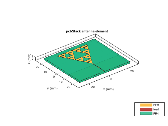

Analyze Return Loss and Gain of Antenna

Manually mesh the antenna structure. The wavelength lambda at the center frequency is 0.0286 m., so set MaxEdgeLength to lambda/8. Eight triangles per wavelength are enough to simulate the structure.

Calculate the wavelength for a resonant frequency of 5 GHz. The relative permittivity of the FR4 is 4.4.

lambda = physconst("lightspeed")/(5e9*sqrt(4.4));
figure
mesh(pcb,MaxEdgeLength=lambda/8);

Use the sparameters function to calculate the S-parameters of the antenna over a frequency range of 2 to 7 GHz. Plot the S-parameters using the rfplot function.

spar = sparameters(pcb,linspace(2e9,7e9,51));
figure
rfplot(spar)

The Modified Sierpinski fractal monopole antenna exhibits its first resonance point centered at 3 GHz, for which the corresponding value of $S_{11}$ is -22.48 dB. The impedance bandwidth for which $S_{11}$ < -10 dB is 2.7 to 3.3 GHz. The second resonance point is centered at 5.2 GHz, for which the corresponding value of $S_{11}$ is -14.5 dB. The impedance bandwidth such that $S_{11}$ < -10 dB is 4.9 to 5.6 GHz.

Plot the radiation pattern of this antenna at the first (3 GHz) and second (5 GHz) resonant frequency. The pattern plots are in the S and C frequency bands, with peak gains of 2.1 dB at 3 GHz and 3.78 dB at 5 GHz.

figure
pattern(pcb,3e9);

figure
pattern(pcb,5e9)

Reference

[1] Islam, Zain Ul, Muhibur Rahman, Niaz Muhammad, Zeeshan Ahmed, Faiz Khalid Lodhi, and Muhammad Haneef. “Dual Band Second Order Modified Sierpinski Monopole Reduced Size Fractal Antenna.” In 2016 International Conference on Emerging Technologies (ICET), 1–5. Islamabad, Pakistan: IEEE, 2016. https://doi.org/10.1109/ICET.2016.7813244.