SADEA Optimization of Six-Element Yagi-Uda Antenna using Custom Objective Function

This example shows how to optimize an antenna design using a custom objective function. The radiation patterns of antennas depend sensitively on the parameters that define the antenna shapes. Typically, the features of a radiation pattern have multiple local optima. The radiation pattern of the antenna is calculated using the pattern function in Antenna Toolbox. The optimization is performed using the optimize method which uses the SADEA optimizer for antennas and a custom objective function.

A Yagi-Uda antenna is a widely used radiating structure for a variety of applications in commercial and military sectors. This antenna can receive TV signals in the VHF-UHF range of frequencies [1]. The Yagi-Uda is a directional traveling-wave antenna with a single driven element, usually a folded dipole or a standard dipole, which is surrounded by several passive dipoles. The passive elements form the reflector and director. These names identify the positions relative to the driven element. The reflector dipole is behind the driven element, in the direction of the back lobe of the antenna radiation. The director dipole is in front of the driven element, in the direction where a main beam forms.

Design Parameters

Specify the initial design parameters for the Yagi-Uda antenna to operate at the center of the VHF band [2] .

freq = 165e6;
wirediameter = 19e-3;
c = physconst("lightspeed");
lambda = c/freq;
Z0 = 300;
BW = 0.05*freq;
fmin = freq - 2*(BW);
fmax = freq + 2*(BW);
Nf = 101;

Create Yagi-Uda Antenna

The driven element for the Yagi-Uda antenna is a folded dipole, a standard exciter for this type of antenna. Adjust the length and width parameters of the folded dipole. Because cylindrical structures are modeled as equivalent metal strips, calculate the width using the cylinder2strip utility function available in the Antenna Toolbox™. The length is $$\lambda /2$$ at the design frequency.

d = dipoleFolded;
d.Length = lambda/2;
d.Width = cylinder2strip(wirediameter/2);
d.Spacing = d.Length/60;

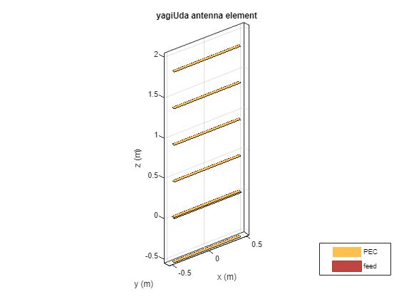
Create a Yagi-Uda antenna with the exciter as the folded dipole. Set the lengths of the reflector and director elements to be $$\lambda /2$$. Set the number of directors to four. Specify the reflector and director spacing as $$0.3\lambda$$ and $$0.25\lambda$$, respectively. These settings provide an initial guess and serve as a starting point for the optimization procedure. View the initial design.

Numdirs = 4;
refLength = 0.5;
dirLength = 0.5*ones(1,Numdirs);
refSpacing = 0.3;
dirSpacing = 0.25*ones(1,Numdirs);
initialdesign = [refLength dirLength refSpacing dirSpacing].*lambda;
yagidesign = yagiUda;
yagidesign.Exciter = d;
yagidesign.NumDirectors = Numdirs;
yagidesign.ReflectorLength = refLength*lambda;
yagidesign.DirectorLength = dirLength.*lambda;
yagidesign.ReflectorSpacing = refSpacing*lambda;
yagidesign.DirectorSpacing = dirSpacing*lambda;
fig = figure;
show(yagidesign)

Plot Radiation Pattern at Design Frequency

Prior to executing the optimization process, plot the radiation pattern for the initial guess in 3-D.

fig1 = figure;
pattern(yagidesign,freq);

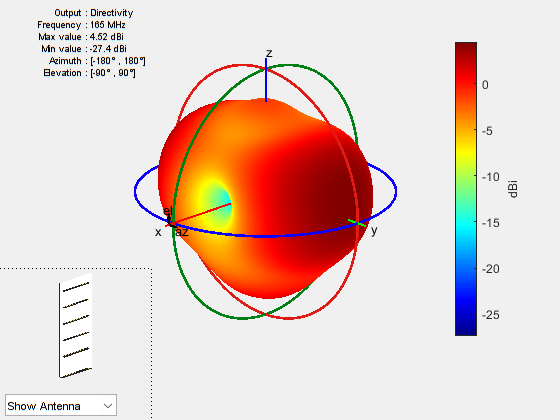
This antenna does not have a higher directivity in the preferred direction, at zenith (elevation = 90 deg). This initial Yagi-Uda antenna design is a poorly designed radiator.

Set Up Optimization

Use the following variables as control variables for the optimization:

• Reflector length (1 variable)

• Director lengths (1 variables)

• Reflector spacing (1 variable)

• Director spacings (1 variables)

The SADEA optimizer sets the values to the corresponding properties of the yagiuda and provides the antenna object as input to the custom objective function.

Create a custom objective function that takes the antenna as input and returns an objective value / penalty as output. The antenna is provided as input to the custom objective by the SADEA optimizer the parameters for the current iteration are set by the optimizer and given as input to the function. The custom objective function aims to have a large value in the 90-degree direction, a small value in the 270-degree direction, and a large value of maximum power between the elevation beamwidth angle bounds.

In addition to the directivity goal an impedance match condition is also included as a constraint. Any constraint violations will penalize the objective.

type yagi_custom_objective_function.m

function objectivevalue = yagi_custom_objective_function(y)
% yagi_custom_objective_function returns the objective for a 6-element Yagi
% objectivevalue = yagi_custom_objective_function(y)
% it calculates the objective value for the yagiUda antenna y passed in as
% input by the SADEA optimizer

% The yagi_custom_objective_function function is used for an internal example.
% Its behavior might change in subsequent releases, so it should not be
% relied upon for programming purposes.

% Copyright 2023-2024 The MathWorks, Inc.
fc = 165e6;
Z0 = 300;
BW = 0.05*fc;
fmin = fc - 2*(BW);
fmax = fc + 2*(BW);
Nf = 101;
freq = linspace(fmin,fmax,Nf);
ang = [0 0;90 -90];  


constraints.S11min = -10;
constraints.Gmin = 10.5;
constraints.Gdeviation = 0.1;
constraints.FBmin = 15;
constraints.Penalty = 50;

% Unpack constraints
Gmin = constraints.Gmin;
Gdev = constraints.Gdeviation;
FBmin = constraints.FBmin;
S11min = constraints.S11min;
K = constraints.Penalty;

% Calculate antenna port and field parameters
output = analyzeAntenna(y,fc,BW,ang,Z0);

% Form objective function
output1 = output.MaxDirectivity+output.MismatchLoss;    % Directivity/Gain at zenith

% Gain constraint, e.g. G > 10
c1 = 0;
if output1<Gmin
    c1 = Gmin-output1;
end

% Gain deviation constraint, abs(G-Gmin)<0.1;
c1_dev = 0;
if abs(output1-Gmin)>Gdev
    c1_dev = -Gdev + abs(output1-Gmin);
end

% Front to Back Ratio constraint, e.g. F/B > 15
c2 = 0;
if output.FB < FBmin
    c2 = FBmin-output.FB;
end

% Reflection Coefficient, S11 < -10
c3 = 0;
if output.S11 > S11min
   c3 = -S11min + output.S11; 
end

% Form the objective + constraints
objectivevalue = -output1 + max(0,(c1+c1_dev+c2+c3))*K;
end

function output = analyzeAntenna(ant,fc,BW,ang,Z0)
%ANALYZEANTENNA calculate the objective function
% OUTPUT = ANALYZEANTENNA(Y,FREQ,BW,ANG,Z0) performs analysis on the
% antenna ANT at the frequency, FC, and calculates the directivity at the
% angles specified by ANG and the front-to-back ratio. The reflection
% coefficient relative to reference impedance Z0, and impedance are
% computed over the bandwidth BW around FC.

fmin = fc - (BW/2);
fmax = fc + (BW/2);
Nf = 5;
freq = unique([fc,linspace(fmin,fmax,Nf)]);
fcIdx = freq==fc;
s = sparameters(ant,freq,Z0);
Z = impedance(ant,fc);
az = ang(1,:);
el = ang(2,:);
Dmax = pattern(ant,fc,az(1),el(1));
Dback = pattern(ant,fc,az(2),el(2));

% Calculate F/B
F_by_B = Dmax-Dback;

% Compute S11 and mismatch loss
s11 = rfparam(s,1,1);
S11 = max(20*log10(abs(s11)));
T = mean(10*log10(1 - (abs(s11)).^2));

% Form the output structure
output.MaxDirectivity= Dmax;
output.BackLobeLevel = Dback;
output.FB = F_by_B;
output.S11 = S11;
output.MismatchLoss = T;
output.Z = Z;
end

Set bounds on the control variables.

refLengthBounds = [0.4;
                    0.6].*lambda;
dirLengthBounds = [0.35 ;   % lower bound on director length
                   0.5].*lambda;  % upper bound on director length
refSpacingBounds = [0.05;                 % lower bound on reflector spacing
                    0.30].*lambda;                % upper bound on reflector spacing
dirSpacingBounds = [0.05 ;  % lower bound on director spacing
                    0.23].*lambda; % upper bound on director spacing

LBUB = {refLengthBounds(1) dirLengthBounds(1) refSpacingBounds(1) dirSpacingBounds(1);
        refLengthBounds(2) dirLengthBounds(2) refSpacingBounds(2) dirSpacingBounds(2) };

SADEA optimization using custom objective

Run the optimization using SADEA. Setup design variables as ReflectorLength, DirectorLength, ReflectorSpacing, DirectorSpacing. Set the number of iterations to 150. Call the optimize method on the yagiuda antenna at the frequency defined by freq, with the options mentioned before.

designVars = {'ReflectorLength','DirectorLength','ReflectorSpacing','DirectorSpacing'};
num_iterations = 150;
fig2 = figure;
optimdesign = optimize(yagidesign, freq, @yagi_custom_objective_function, designVars, LBUB, 'Iterations', num_iterations );

The optimization stopped because it reached the num iterations.

Initial Objective Value

initialObjectiveValue = yagi_custom_objective_function(yagidesign)

initialObjectiveValue = 2.5910e+03

Final Objective Value

finalObjectiveValue = yagi_custom_objective_function(optimdesign)

finalObjectiveValue = -10.5751

SADEA found an antenna with objective value of 56. The overall penalty is reduced from 2600 to 56.

Plot Optimized Pattern

Plot the optimized antenna pattern at the design frequency.

yagidesign = optimdesign;
fig3 = figure;
pattern(yagidesign,freq)

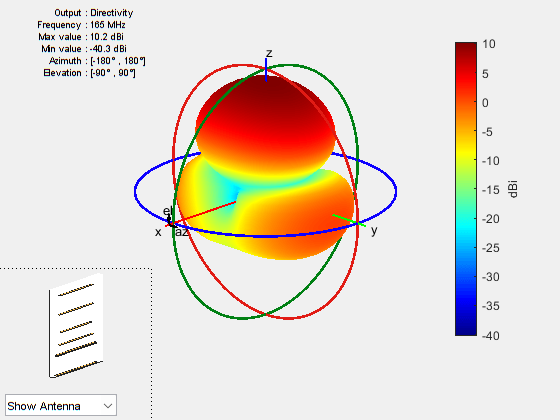
Apparently, the antenna now radiates significantly more power at zenith.

E-Plane and H-Plane Cuts of Pattern

To obtain a better insight into the behavior in two orthogonal planes, plot the normalized magnitude of the electric field in the E-plane and H-plane, that is, azimuth = 0 and 90 deg, respectively.

fig4 = figure;
pattern(yagidesign,freq,0,0:1:359);

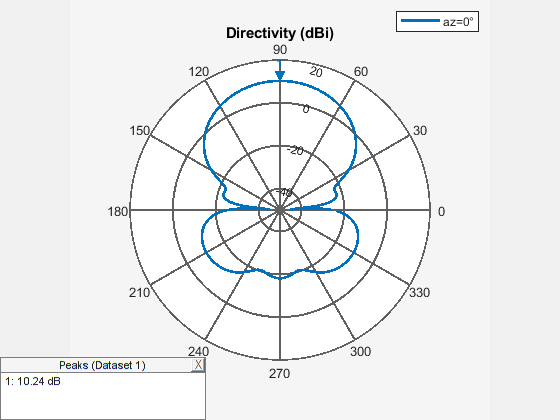
fig5 = figure;
pattern(yagidesign,freq,90,0:1:359);

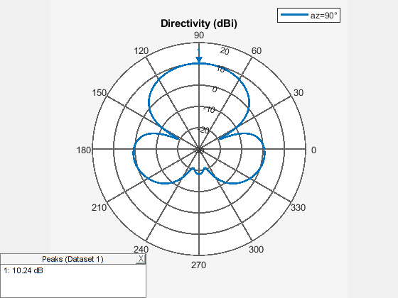
The optimized design shows a significant improvement in the radiation pattern. Higher directivity is achieved in the desired direction toward zenith. The back lobe is small, resulting in a good front-to-back ratio for this antenna. Calculate the directivity at zenith, front-to-back ratio, and beamwidth in the E-plane and H-plane.

D_max = pattern(yagidesign,freq,0,90)

D_max = 10.7895

D_back = pattern(yagidesign,freq,0,-90)

D_back = -7.8695

F_B_ratio = D_max - D_back

F_B_ratio = 18.6589

Eplane_beamwidth = beamwidth(yagidesign,freq,0,1:1:360)

Eplane_beamwidth = 54

Hplane_beamwidth = beamwidth(yagidesign,freq,90,1:1:360)

Hplane_beamwidth = 66.0000

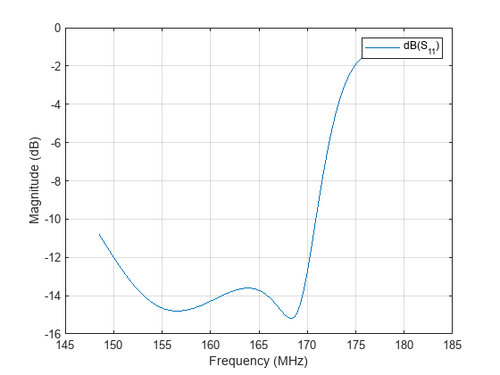
Input Reflection Coefficient of Optimized Antenna

Choose initial design parameters for the Yagi-Uda antenna to operate at the center of the VHF band [2]. The datasheet lists a 50Ω input impedance after taking into account a balun. Our model does not account for the presence of the balun and therefore will match to the typical folded dipole input impedance of 300Ω.

freqRange = linspace(fmin,fmax,Nf);
s = sparameters(yagidesign,freqRange,Z0);
fig6 = figure;
rfplot(s);

Comparison with Manufacturer Data Sheet

The optimized Yagi-Uda antenna achieves a forward directivity greater than 10 dBi, which translates to a value greater than 8 dBd (relative to a dipole). This is close to the gain value reported by the datasheet (8.5 dBd). The F/B ratio is13 dB which is slightly lesser than desired. The optimized Yagi-Uda antenna has a E-plane and H-plane beamwidth that compare favorably to the datasheet listed values of 52 degrees and 64 degrees respectively. The design achieves a good impedance match to $$300\Omega$$, and has a -10 dB bandwidth of approximately 10%.

datasheetparam = {'Gain (dBi)';'F/B';'E-plane Beamwidth (deg.)';'H-plane Beamwidth (deg.)';'Impedance Bandwidth (%)'};
datasheetvals = [10.5,16,54,63,10]';
optimdesignvals = [10.81,13,52,64,10]';
Tdatasheet = table(datasheetvals,optimdesignvals,RowNames=datasheetparam)

Tdatasheet=5×2 table
                                datasheetvals    optimdesignvals
                                _____________    _______________

    Gain (dBi)                      10.5              10.81     
    F/B                               16                 13     
    E-plane Beamwidth (deg.)          54                 52     
    H-plane Beamwidth (deg.)          63                 64     
    Impedance Bandwidth (%)           10                 10     

Tabulate Initial and Optimized Design Parameters

Tabulate the initial design guesses and the final optimized design values.

yagiparam=  {'Reflector Length';
             'Director Length - 1'; 'Director Length - 2';
             'Director Length - 3'; 'Director Length - 4';
             'Reflector Spacing'; 'Director Spacing - 1';
             'Director Spacing - 2'; 'Director Spacing - 3';
             'Director Spacing - 4'};         
initialdesignVal = initialdesign';
optimdesignVal = [optimdesign.ReflectorLength optimdesign.DirectorLength optimdesign.ReflectorSpacing optimdesign.DirectorSpacing]';
Tgeometry = table(initialdesignVal,optimdesignVal,RowNames=yagiparam)

Tgeometry=10×2 table
                            initialdesignVal    optimdesignVal
                            ________________    ______________

    Reflector Length            0.90846            0.90745    
    Director Length - 1         0.90846            0.80294    
    Director Length - 2         0.90846             0.7599    
    Director Length - 3         0.90846            0.74138    
    Director Length - 4         0.90846            0.71345    
    Reflector Spacing           0.54508            0.39347    
    Director Spacing - 1        0.45423            0.15914    
    Director Spacing - 2        0.45423            0.31443    
    Director Spacing - 3        0.45423            0.39287    
    Director Spacing - 4        0.45423            0.40161    

Reference

[1] Balanis, Constantine A. Antenna Theory: Analysis and Design. Fourth edition. Hoboken, New Jersey: Wiley, 2016.

[2] Online at: https://amphenolprocom.com/products/base-station-antennas/2450-s-6y-165