Predicting Protein Secondary Structure Using a Neural Network

This example uses:

This example shows a secondary structure prediction method that uses a feed-forward neural network and the functionality available with the Deep Learning Toolbox™.

It is a simplified example intended to illustrate the steps for setting up a neural network with the purpose of predicting secondary structure of proteins. Its configuration and training methods are not meant to be necessarily the best solution for the problem at hand.

Introduction

Neural network models attempt to simulate the information processing that occurs in the brain and are widely used in a variety of applications, including automated pattern recognition.

The Rost-Sander data set [1] consists of proteins whose structures span a relatively wide range of domain types, composition and length. The file RostSanderDataset.mat contains a subset of this data set, where the structural assignment of every residue is reported for each protein sequence.

load RostSanderDataset.mat

N = numel(allSeq);

id = allSeq(7).Header            % annotation of a given protein sequence
seq = int2aa(allSeq(7).Sequence) % protein sequence
str = allSeq(7).Structure        % structural assignment

id =

    '1CSE-ICOMPLEX(SERINEPROTEINASE-INHIBITOR)03-JU'


seq =

    'KSFPEVVGKTVDQAREYFTLHYPQYNVYFLPEGSPVTLDLRYNRVRVFYNPGTNVVNHVPHVG'


str =

    'CCCHHHCCCCHHHHHHHHHHHCCCCEEEEEECCCCEECCCCCCEEEEEEECCCCEECCCCEEC'

In this example, you will build a neural network to learn the structural state (helix, sheet or coil) of each residue in a given protein, based on the structural patterns observed during a training phase. Due to the random nature of some steps in the following approach, numeric results might be slightly different every time the network is trained or a prediction is simulated. To ensure reproducibility of the results, we reset the global random generator to a saved state included in the loaded file, as shown below:

rng(savedState);

Defining the Network Architecture

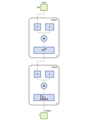
For the current problem we define a neural network with one input layer, one hidden layer and one output layer. The input layer encodes a sliding window in each input amino acid sequence, and a prediction is made on the structural state of the central residue in the window. We choose a window of size 17 based on the statistical correlation found between the secondary structure of a given residue position and the eight residues on either side of the prediction point [2]. Each window position is encoded using a binary array of size 20, having one element for each amino acid type. In each group of 20 inputs, the element corresponding to the amino acid type in the given position is set to 1, while all other inputs are set to 0. Thus, the input layer consists of R = 17x20 input units, i.e. 17 groups of 20 inputs each.

In the following code, we first determine for each protein sequence all the possible subsequences corresponding to a sliding window of size W by creating a Hankel matrix, where the ith column represents the subsequence starting at the ith position in the original sequence. Then for each position in the window, we create an array of size 20, and we set the jth element to 1 if the residue in the given position has a numeric representation equal to j.

W = 17; % sliding window size


% === binarization of the inputs
for i = 1:N
	seq = double(allSeq(i).Sequence);   % current sequence
	win = hankel(seq(1:W),seq(W:end));  % all possible sliding windows
	myP = zeros(20*W,size(win,2));      % input matrix for current sequence
	for k = 1:size(win, 2)
		index = 20*(0:W-1)' + win(:,k); % input array for each position k
		myP(index,k) = 1;
	end
	allSeq(i).P = myP;
end

The output layer of our neural network consists of three units, one for each of the considered structural states (or classes), which are encoded using a binary scheme. To create the target matrix for the neural network, we first obtain, from the data, the structural assignments of all possible subsequences corresponding to the sliding window. Then we consider the central position in each window and transform the corresponding structural assignment using the following binary encoding: 1 0 0 for coil, 0 1 0 for sheet, 0 0 1 for helix.

cr = ceil(W/2); % central residue position

% === binarization of the targets
for i = 1:N
	str = double(allSeq(i).Structure); % current structural assignment
    win = hankel(str(1:W),str(W:end)); % all possible sliding windows
	myT = false(3,size(win,2));
	myT(1,:) = win(cr,:) == double('C');
	myT(2,:) = win(cr,:) == double('E');
	myT(3,:) = win(cr,:) == double('H');
	allSeq(i).T = myT;
end

You can perform the binarization of the input and target matrix described in the two steps above in a more concise way by executing the following equivalent code:

% === concise binarization of the inputs and targets
for i = 1:N
	seq = double(allSeq(i).Sequence);
    win = hankel(seq(1:W),seq(W:end)); % concurrent inputs (sliding windows)

	% === binarization of the input matrix
	allSeq(i).P = kron(win,ones(20,1)) == kron(ones(size(win)),(1:20)');

	% === binarization of the target matrix
	allSeq(i).T = allSeq(i).Structure(repmat((W+1)/2:end-(W-1)/2,3,1)) == ...
		 repmat(('CEH')',1,length(allSeq(i).Structure)-W+1);
end

Once we define the input and target matrices for each sequence, we create an input matrix, P, and target matrix, T, representing the encoding for all the sequences fed into the network.

% === construct input and target matrices
P = double([allSeq.P]); % input matrix
T = double([allSeq.T]); % target matrix

Creating the Neural Network

The problem of secondary structure prediction can be thought of as a pattern recognition problem, where the network is trained to recognize the structural state of the central residue most likely to occur when specific residues in the given sliding window are observed. We create a pattern recognition neural network using the input and target matrices defined above and specifying a hidden layer of size 3.

hsize = 3;
net = patternnet(hsize);
net.layers{1} % hidden layer
net.layers{2} % output layer

ans = 

    Neural Network Layer
 
              name: 'Hidden'
        dimensions: 3
       distanceFcn: (none)
     distanceParam: (none)
         distances: []
           initFcn: 'initnw'
       netInputFcn: 'netsum'
     netInputParam: (none)
         positions: []
             range: [3x2 double]
              size: 3
       topologyFcn: (none)
       transferFcn: 'tansig'
     transferParam: (none)
          userdata: (your custom info)
 

ans = 

    Neural Network Layer
 
              name: 'Output'
        dimensions: 0
       distanceFcn: (none)
     distanceParam: (none)
         distances: []
           initFcn: 'initnw'
       netInputFcn: 'netsum'
     netInputParam: (none)
         positions: []
             range: []
              size: 0
       topologyFcn: (none)
       transferFcn: 'softmax'
     transferParam: (none)
          userdata: (your custom info)

Training the Neural Network

The pattern recognition network uses the default Scaled Conjugate Gradient algorithm for training, but other algorithms are available (see the Deep Learning Toolbox documentation for a list of available functions). At each training cycle, the training sequences are presented to the network through the sliding window defined above, one residue at a time. Each hidden unit transforms the signals received from the input layer by using a transfer function logsig to produce an output signal that is between and close to either 0 or 1, simulating the firing of a neuron [2]. Weights are adjusted so that the error between the observed output from each unit and the desired output specified by the target matrix is minimized.

% === use the log sigmoid as transfer function
net.layers{1}.transferFcn = 'logsig';

% === train the network
[net,tr] = train(net,P,T);

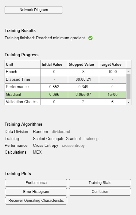
During training, the training tool window opens and displays the progress. Training details such as the algorithm, the performance criteria, the type of error considered, etc. are shown.

Use the function view to generate a graphical view of the neural network.

view(net)

One common problem that occurs during neural network training is data overfitting, where the network tends to memorize the training examples without learning how to generalize to new situations. The default method for improving generalization is called early stopping and consists in dividing the available training data set into three subsets: (i) the training set, which is used for computing the gradient and updating the network weights and biases; (ii) the validation set, whose error is monitored during the training process because it tends to increase when data is overfitted; and (iii) the test set, whose error can be used to assess the quality of the division of the data set.

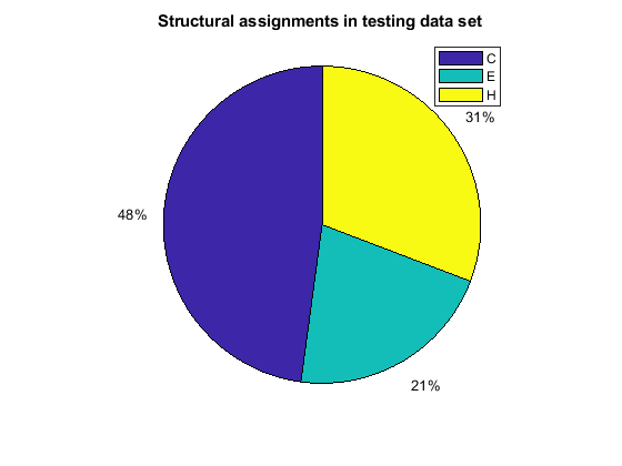
When using the function train, by default, the data is randomly divided so that 60% of the samples are assigned to the training set, 20% to the validation set, and 20% to the test set, but other types of partitioning can be applied by specifying the property net.divideFnc (default dividerand). The structural composition of the residues in the three subsets is comparable, as seen from the following survey:

[i,j] = find(T(:,tr.trainInd));
Ctrain = sum(i == 1)/length(i);
Etrain = sum(i == 2)/length(i);
Htrain = sum(i == 3)/length(i);

[i,j] = find(T(:,tr.valInd));
Cval = sum(i == 1)/length(i);
Eval = sum(i == 2)/length(i);
Hval = sum(i == 3)/length(i);

[i,j] = find(T(:,tr.testInd));
Ctest = sum(i == 1)/length(i);
Etest = sum(i == 2)/length(i);
Htest = sum(i == 3)/length(i);

figure()
pie([Ctrain; Etrain; Htrain]);
title('Structural assignments in training data set');
legend('C', 'E', 'H')

figure()
pie([Cval; Eval; Hval]);
title('Structural assignments in validation data set');
legend('C', 'E', 'H')

figure()
pie([Ctest; Etest; Htest]);
title('Structural assignments in testing data set ');
legend('C', 'E', 'H')

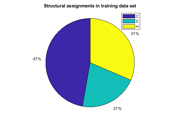
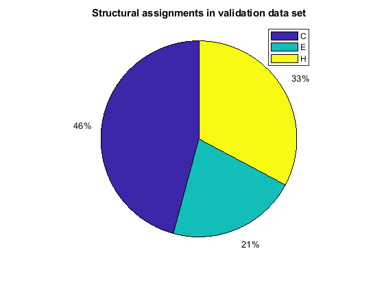
The function plotperform display the trends of the training, validation, and test errors as training iterations pass.

figure()
plotperform(tr)

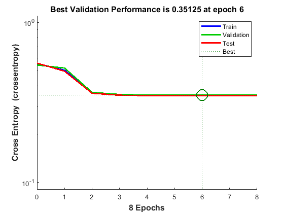
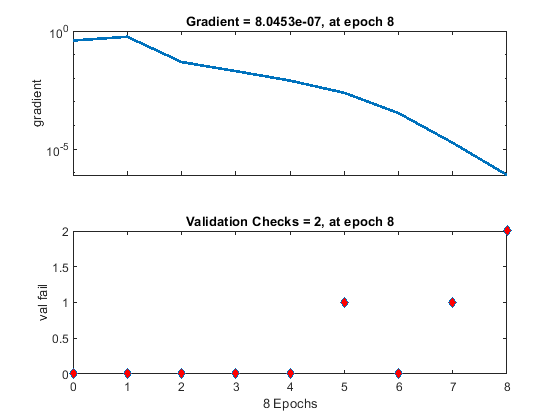
The training process stops when one of several conditions (see net.trainParam) is met. For example, in the training considered, the training process stops when the validation error increases for a specified number of iterations (6) or the maximum number of allowed iterations is reached (1000).

% === display training parameters
net.trainParam

% === plot validation checks and gradient
figure()
plottrainstate(tr)

ans = 

 
    Function Parameters for 'trainscg'
 
    Show Training Window Feedback   showWindow: true
    Show Command Line Feedback showCommandLine: false
    Command Line Frequency                show: 25
    Maximum Epochs                      epochs: 1000
    Maximum Training Time                 time: Inf
    Performance Goal                      goal: 0
    Minimum Gradient                  min_grad: 1e-06
    Maximum Validation Checks         max_fail: 6
    Sigma                                sigma: 5e-05
    Lambda                              lambda: 5e-07

Analyzing the Network Response

To analyze the network response, we examine the confusion matrix by considering the outputs of the trained network and comparing them to the expected results (targets).

O = sim(net,P);
figure()
plotconfusion(T,O);

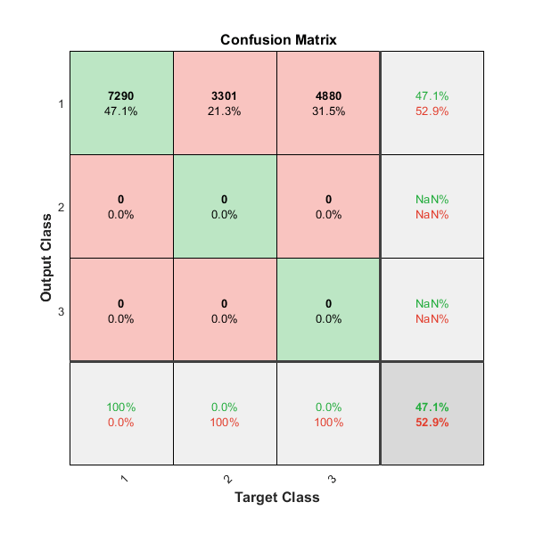
The diagonal cells show the number of residue positions that were correctly classified for each structural class. The off-diagonal cells show the number of residue positions that were misclassified (e.g. helical positions predicted as coiled positions). The diagonal cells correspond to observations that are correctly classified. Both the number of observations and the percentage of the total number of observations are shown in each cell. The column on the far right of the plot shows the percentages of all the examples predicted to belong to each class that are correctly and incorrectly classified. These metrics are often called the precision (or positive predictive value) and false discovery rate, respectively. The row at the bottom of the plot shows the percentages of all the examples belonging to each class that are correctly and incorrectly classified. These metrics are often called the recall (or true positive rate) and false negative rate, respectively. The cell in the bottom right of the plot shows the overall accuracy.

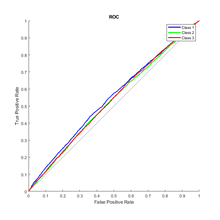
We can also consider the Receiver Operating Characteristic (ROC) curve, a plot of the true positive rate (sensitivity) versus the false positive rate (1 - specificity).

figure()
plotroc(T,O);

Refining the Neural Network for More Accurate Results

The neural network that we have defined is relative simple. To achieve some improvements in the prediction accuracy we could try one of the following:

Increase the number of training vectors. Increasing the number of sequences dedicated to training requires a larger curated database of protein structures, with an appropriate distribution of coiled, helical and sheet elements.
Increase the number of input values. Increasing the window size or adding more relevant information, such as biochemical properties of the amino acids, are valid options.
Use a different training algorithm. Various algorithms differ in memory and speed requirements. For example, the Scaled Conjugate Gradient algorithm is relatively slow but memory efficient, while the Levenberg-Marquardt is faster but more demanding in terms of memory.
Increase the number of hidden neurons. By adding more hidden units we generally obtain a more sophisticated network with the potential for better performances but we must be careful not to overfit the data.

We can specify more hidden layers or increased hidden layer size when the pattern recognition network is created, as shown below:

hsize = [3 4 2];
net3 = patternnet(hsize);

hsize = 20;
net20 = patternnet(hsize);

We can also assign the network initial weights to random values in the range -0.1 to 0.1 as suggested by the study reported in [2] by setting the net20.IW and net20.LW properties as follows:

% === assign random values in the range -.1 and .1 to the weights
net20.IW{1} = -.1 + (.1 + .1) .* rand(size(net20.IW{1}));
net20.LW{2} = -.1 + (.1 + .1) .* rand(size(net20.LW{2}));

In general, larger networks (with 20 or more hidden units) achieve better accuracy on the protein training set, but worse accuracy in the prediction accuracy. Because a 20-hidden-unit network involves almost 7,000 weights and biases, the network is generally able to fit the training set closely but loses the ability of generalization. The compromise between intensive training and prediction accuracy is one of the fundamental limitations of neural networks.

net20 = train(net20,P,T);

O20 = sim(net20,P);
numWeightsAndBiases = length(getx(net20))

numWeightsAndBiases =

        6883

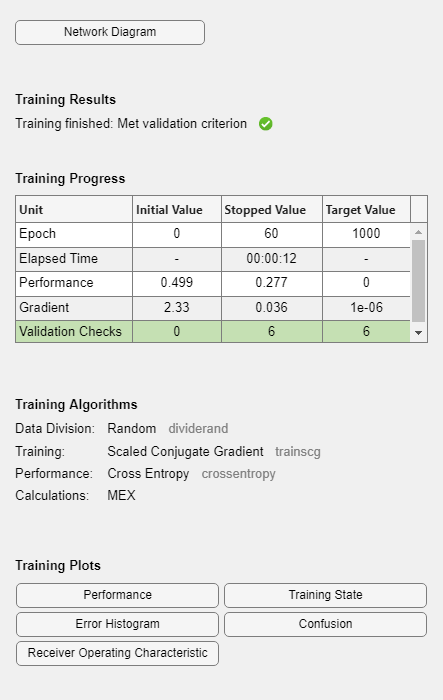
You can display the confusion matrices for training, validation and test subsets by clicking on the corresponding button in the training tool window.

Assessing Network Performance

You can evaluate structure predictions in detail by calculating prediction quality indices [3], which indicate how well a particular state is predicted and whether overprediction or underprediction has occurred. We define the index pcObs(S) for state S (S = {C, E, H}) as the number of residues correctly predicted in state S, divided by the number of residues observed in state S. Similarly, we define the index pcPred(S) for state S as the number of residues correctly predicted in state S, divided by the number of residues predicted in state S.

[i,j] = find(compet(O));
[u,v] = find(T);

% === compute fraction of correct predictions when a given state is observed
pcObs(1) = sum(i == 1 & u == 1)/sum (u == 1); % state C
pcObs(2) = sum(i == 2 & u == 2)/sum (u == 2); % state E
pcObs(3) = sum(i == 3 & u == 3)/sum (u == 3); % state H

% === compute fraction of correct predictions when a given state is predicted
pcPred(1) = sum(i == 1 & u == 1)/sum (i == 1); % state C
pcPred(2) = sum(i == 2 & u == 2)/sum (i == 2); % state E
pcPred(3) = sum(i == 3 & u == 3)/sum (i == 3); % state H

% === compare quality indices of prediction
figure()
bar([pcObs' pcPred'] * 100);
ylabel('Correctly predicted positions (%)');
ax = gca;
ax.XTickLabel = {'C';'E';'H'};
legend({'Observed','Predicted'});

These quality indices are useful for the interpretation of the prediction accuracy. In fact, in cases where the prediction technique tends to overpredict/underpredict a given state, a high/low prediction accuracy might just be an artifact and does not provide a measure of quality for the technique itself.

Conclusions

The method presented here predicts the structural state of a given protein residue based on the structural state of its neighbors. However, there are further constraints when predicting the content of structural elements in a protein, such as the minimum length of each structural element. Specifically, a helix is assigned to any group of four or more contiguous residues, and a sheet is assigned to any group of two or more contiguous residues. To incorporate this type of information, an additional network can be created so that the first network predicts the structural state from the amino acid sequence, and the second network predicts the structural element from the structural state.

References

[1] Rost, B., and Sander, C., "Prediction of protein secondary structure at better than 70% accuracy", Journal of Molecular Biology, 232(2):584-99, 1993.

[2] Holley, L.H. and Karplus, M., "Protein secondary structure prediction with a neural network", PNAS, 86(1):152-6, 1989.

[3] Kabsch, W., and Sander, C., "How good are predictions of protein secondary structure?", FEBS Letters, 155(2):179-82, 1983.