Adaptive Equalizers
Adaptive equalizer structures provide suboptimal equalization of time variations in the propagation channel characteristics. However, these equalizers are appealing because their computational complexity is lower than MLSE Equalizers.
In Communications Toolbox™, the comm.LinearEqualizer
and comm.DecisionFeedbackEqualizer System objects and the Linear Equalizer and
Decision Feedback
Equalizer blocks use tap delay line filters to equalize a linearly modulated signal
through a dispersive channel. These features output the estimate of the signal by using an
estimate of the channel modeled as a finite input response (FIR) filter.
To decode a received signal, the adaptive equalizer:
Applies the FIR filter to the symbols in the input signal. The FIR filter tap weights correspond to the channel estimate.
Outputs the signal estimate and uses the signal estimate to update the tap weights for the next symbol. The signal estimate and updating of weights depends on the adaptive equalizer structure and algorithm.
Adaptive equalizer structure options are linear or decision-feedback. Adaptive algorithm options are least mean square (LMS), recursive mean square (RMS), or constant modulus algorithm (CMA). For background material on adaptive equalizers, see Selected References for Equalizers.
Number of Taps
For the linear equalizer, the number of taps must be greater than or equal to the number of input samples per symbol. For the decision feedback equalizer, the number of forward taps must be greater than or equal to the number of input samples per symbol.
Symbol Tap Spacing
You can configure the equalizer to operate as a symbol-spaced equalizer or as a fractional symbol-spaced equalizer.
To operate the equalizer at a symbol-spaced rate, specify the number of samples per symbol as
1. Symbol-rate equalizers have taps spaced at the symbol duration. Symbol-rate equalizers are sensitive to timing phase.To operate the equalizer at a fractional symbol-spaced rate, specify the number of input samples per symbol as an integer greater than
1and provide an input signal oversampled at that sampling rate. Fractional symbol-spaced equalizers have taps spaced at an integer fraction of the input symbol duration. Fractional symbol-spaced equalizers are not sensitive to timing phase.
Note
The MLSE equalizer supports fractional symbol spacing but using it is not recommended. The MLSE computational complexity and burden grows exponentially with the length of the channel time dispersion. Oversampling the input means multiplying the exponential term by the number of samples per symbol.
Linear Equalizers
Linear equalizers can remove intersymbol interference (ISI) when the frequency response of a channel has no null. If a null exists in the frequency response of a channel, linear equalizers tend to enhance the noise. In this case, use decision feedback equalizers to avoid enhancing the noise.
A linear equalizer consists of a tapped delay line that stores samples from the input signal. Once per symbol period, the equalizer outputs a weighted sum of the values in the delay line and updates the weights to prepare for the next symbol period.
Linear equalizers can be symbol-spaced or fractional symbol-spaced.
For a symbol-spaced equalizer, the number of samples per symbol, K, is 1. The output sample rate equals the input sample rate.
For a fractional symbol-spaced equalizer, the number of samples per symbol, K, is an integer greater than 1. Typically, K is 4 for fractionally spaced equalizers. The output sample rate is 1/T and the input sample rate is K/T, where T is the symbol period. Tap-weight updating occurs at the output rate.
This schematic shows a linear equalizer with L weights, a symbol period of T, and K samples per symbol. If K is 1, the result is a symbol-spaced linear equalizer instead of a fractional symbol-spaced linear equalizer.

In each symbol period, the equalizer receives K input samples at the tapped delay line. The equalizer then outputs a weighted sum of the values in the tapped delay line and updates the weights to prepare for the next symbol period.
Decision-Feedback Equalizers
A decision feedback equalizer (DFE) is a nonlinear equalizer that reduces intersymbol interference (ISI) in frequency-selective channels. If a null exists in the frequency response of a channel, DFEs do not enhance the noise. A DFE consists of a tapped delay line that stores samples from the input signal and contains a forward filter and a feedback filter. The forward filter is similar to a linear equalizer. The feedback filter contains a tapped delay line whose inputs are the decisions made on the equalized signal. Once per symbol period, the equalizer outputs a weighted sum of the values in the delay line and updates the weights to prepare for the next symbol period.
DFEs can be symbol-spaced or fractional symbol-spaced.
For a symbol-spaced equalizer, the number of samples per symbol, K, is 1. The output sample rate equals the input sample rate.
For a fractional symbol-spaced equalizer, the number of samples per symbol, K, is an integer greater than 1. Typically, K is 4 for fractional symbol-spaced equalizers. The output sample rate is 1/T and the input sample rate is K/T. Tap weight updating occurs at the output rate.
This schematic shows a fractional symbol-spaced DFE with a total of N weights, a symbol period of T, and K samples per symbol. The filter has L forward weights and N-L feedback weights. The forward filter is at the top, and the feedback filter is at the bottom. If K is 1, the result is a symbol-spaced DFE instead of a fractional symbol-spaced DFE.

In each symbol period, the equalizer receives K input samples at the forward filter and one decision or training sample at the feedback filter. The equalizer then outputs a weighted sum of the values in the forward and feedback delay lines and updates the weights to prepare for the next symbol period.
Note
The algorithm for the Adaptive Algorithm block in the schematic jointly optimizes the forward and feedback weights. Joint optimization is especially important for convergence in the recursive least square (RLS) algorithm.
Reference Signal and Operating Modes
In default applications, the equalizer first operates in training mode to gather information about the channel. The equalizer later switches to decision-directed mode.
When the equalizer is operating in training mode, the reference signal is a preset, known transmitted sequence.
When the equalizer is operating in decision-directed mode, the reference signal is a detected version of the output signal, denoted by yd in the schematic.
The CMA algorithm has no training mode. Training mode applies only when the equalizer is configured to use the LMS or RLS algorithm.
Error Calculation
The error calculation operation produces a signal given by this expression, where R is a constant related to the signal constellation.
Updating Tap Weights
For linear and decision-feedback equalizer structures, the choice of LMS, RLS, or CMA determines the algorithms that are used to set the tap weights and perform the error calculation. The new set of tap weights depends on:
The current set of tap weights
The input signal
The output signal
The reference signal, d, for LMS and RLS adaptive algorithms only. The reference signal characteristics depend on the operating mode of the equalizer.
Least Mean Square Algorithm
For the LMS algorithm, in the previous schematic, w is a vector of all weights wi, and u is a vector of all inputs ui. Based on the current set of weights, the LMS algorithm creates the new set of weights as
wnew = wcurrent + (StepSize) ue*.
The step size used by the adaptive algorithm is specified as a positive scalar. Increasing the
step size reduces the equalizer convergence time but causes the equalized output signal to
be less stable. To determine the maximum step size allowed when using the LMS adaptive
algorithm, use the maxstep object
function. The * operator denotes the complex conjugate and the error calculation e = d -
y.
Recursive Least Square Algorithm
For the RLS algorithm, in the previous schematic, w is the vector of all weights wi, and u is the vector of all inputs ui. Based on the current set of inputs, u, and the inverse correlation matrix, P, the RLS algorithm first computes the Kalman gain vector, K, as
The forgetting factor used by the adaptive algorithm is specified as a scalar in the range (0, 1]. Decreasing the forgetting factor reduces the equalizer convergence time but causes the equalized output signal to be less stable. H denotes the Hermitian transpose. Based on the current inverse correlation matrix, the new inverse correlation matrix is
Based on the current set of weights, the RLS algorithm creates the new set of weights as
wnew = wcurrent+K*e.
The * operator denotes the complex conjugate and the error calculation e = d - y.
Constant Modulus Algorithm
For the CMA adaptive algorithm, in the previous schematic, w is the vector of all weights wi, and u is the vector of all inputs ui. Based on the current set of weights, the CMA adaptive algorithm creates the new set of weights as
wnew = wcurrent + (StepSize) u*e.
The step size used by the adaptive algorithm is specified as a positive scalar. Increasing the
step size reduces the equalizer convergence time but causes the equalized output signal to
be less stable. To determine the maximum step size allowed by the CMA adaptive algorithm,
use the maxstep object
function. The * operator denotes the complex conjugate and the error calculation
e = y(R -
|y|2), where R is a constant related to the signal
constellation.
Configuring Adaptive Equalizers
Choose the linear or decision-feedback equalizer structure. Decide which adaptive algorithm to use — LMS, RLS, or CMA. Specify settings for structure and algorithm-specific operation modes.
Configuring an equalizer involves selecting a linear or decision-feedback structure, selecting an adaptive algorithm, and specifying the structure and algorithm specific operation modes.
When deciding which adaptive algorithm best fits your needs, consider:
The LMS algorithm executes quickly but converges slowly. Its complexity grows linearly with the number of weights.
The RLS algorithm converges quickly. Its complexity grows approximately with the square of the number of weights. This algorithm can also be unstable when the number of weights is large.
The constant modulus algorithm (CMA) is useful when no training signal is available. It works best for constant modulus modulations such as PSK.
If CMA has no additional side information, it can introduce phase ambiguity. For example, the weights found by the CMA might produce a perfect QPSK constellation but introduce a phase rotation of 90, 180, or 270 degrees. In this case, employ a phase ambiguity correction algorithm or choose a differential modulation scheme. Differential modulation schemes are insensitive to phase ambiguity.
To view or change any properties of an adaptive equalizer, use the syntax described for channel objects in Displaying and Changing Object Properties.
For more information about adaptive algorithms, see the references listed in Selected References for Equalizers.
Specify an Adaptive Equalizer
To create an adaptive equalizer object for use in MATLAB®, select the comm.LinearEqualizer or comm.DecisionFeedbackEqualizer
System object™. For Simulink®, use the Linear Equalizer
or Decision Feedback
Equalizer block. Based on the propagation channel characteristics in your
simulation, use the criteria in Equalization to select the equalizer
structure.
The equalizer object has many properties that record information about the equalizer. Properties can be related to:
The structure of the equalizer, such as the number of taps.
The adaptive algorithm that the equalizer uses, such as the step size in the LMS or CMA algorithm.
Information about the current state of the equalizer. The equalizer object can output the values of the weights.
To view or change any properties of an equalizer object, use the syntax described for channel objects in Displaying and Changing Object Properties.
Defining Equalizer Objects
The code creates equalizer objects for these configurations:
A symbol-spaced linear RLS equalizer with 10 weights.
A fractionally spaced linear RLS equalizer with 10 weights, a BPSK constellation, and two samples per symbol.
A decision-feedback RLS equalizer with three weights in the feedforward filter and two weights in the feedback filter.
All three equalizer objects specify the RLS adaptive algorithm with a forgetting factor of 0.3.
Create equalizer objects of different types. The default settings are used for properties not set using 'Name,Value' pairs.
eqlin = comm.LinearEqualizer( ...
    Algorithm='RLS', ...
    NumTaps=10, ...
    ForgettingFactor=0.3)
eqlin =
  comm.LinearEqualizer with properties:

                          Algorithm: 'RLS'
                            NumTaps: 10
                   ForgettingFactor: 0.3000
    InitialInverseCorrelationMatrix: 0.1000
                      Constellation: [0.7071 + 0.7071i -0.7071 + 0.7071i -0.7071 - 0.7071i 0.7071 - 0.7071i]
                       ReferenceTap: 3
                         InputDelay: 0
              InputSamplesPerSymbol: 1
              TrainingFlagInputPort: false
                 AdaptAfterTraining: true
               InitialWeightsSource: 'Auto'
                 WeightUpdatePeriod: 1
eqfrac = comm.LinearEqualizer( ...
    Algorithm='RLS', ...
    NumTaps=10, ...
    ForgettingFactor=0.3, ...
    Constellation=[-1 1], ...
    InputSamplesPerSymbol=2)
eqfrac =
  comm.LinearEqualizer with properties:

                          Algorithm: 'RLS'
                            NumTaps: 10
                   ForgettingFactor: 0.3000
    InitialInverseCorrelationMatrix: 0.1000
                      Constellation: [-1 1]
                       ReferenceTap: 3
                         InputDelay: 0
              InputSamplesPerSymbol: 2
              TrainingFlagInputPort: false
                 AdaptAfterTraining: true
               InitialWeightsSource: 'Auto'
                 WeightUpdatePeriod: 1
eqdfe = comm.DecisionFeedbackEqualizer( ...
    Algorithm='RLS', ...
    NumForwardTaps=3, ...
    NumFeedbackTaps=2, ...
    ForgettingFactor=0.3)
eqdfe =
  comm.DecisionFeedbackEqualizer with properties:

                          Algorithm: 'RLS'
                     NumForwardTaps: 3
                    NumFeedbackTaps: 2
                   ForgettingFactor: 0.3000
    InitialInverseCorrelationMatrix: 0.1000
                      Constellation: [0.7071 + 0.7071i -0.7071 + 0.7071i -0.7071 - 0.7071i 0.7071 - 0.7071i]
                       ReferenceTap: 3
                         InputDelay: 0
              InputSamplesPerSymbol: 1
              TrainingFlagInputPort: false
                 AdaptAfterTraining: true
               InitialWeightsSource: 'Auto'
                 WeightUpdatePeriod: 1
Adaptive Algorithm Assignment
Use the Algorithm property to assign the adaptive algorithm used by the equalizer.
Algorithm Assignment
When creating the equalizer object, assign the adaptive algorithm.
eqlms = comm.LinearEqualizer('Algorithm','LMS');
Create the equalizer object with default property settings. LMS is the default adaptive algorithm.
eqrls = comm.LinearEqualizer;
eqrls.Algorithm
ans =
'LMS'
Update eqrls to use the RLS adaptive algorithm.
eqrls.Algorithm = 'RLS';
eqrls.Algorithm
ans = 'RLS'
Cloning and Duplicating Objects
Configure a new equalizer object by cloning an existing equalizer object, and then changing its properties. Clone eqlms to create an independent equalizer, eqcma, then update the algorithm to 'CMA'.
eqcma = clone(eqlms);
eqcma.Algorithm
ans =
'LMS'
eqcma.Algorithm = 'CMA';
eqcma.Algorithm
ans = 'CMA'
If you want an independent duplicate, use the clone command.
eqlms.NumTaps
ans =
5
eq2 = eqlms;
eq2.NumTaps = 6;
eq2.NumTaps
ans =
6
eqlms.NumTaps
ans =
6
The clone command creates a copy of eqlms that is independent of eqlms. By contrast, the command eqB = eqA creates eqB as a reference to eqA, so that eqB and eqA always have identical property settings.
Equalizer Training
Linearly Equalize System by Using Different Training Schemes
Demonstrate linear equalization by using the least mean squares (LMS) algorithm to recover QPSK symbols passed through an AWGN channel. Apply different equalizer training schemes and show the symbol error magnitude.
System Setup
Simulate a QPSK-modulated system subject to AWGN. Transmit packets composed of 200 training symbols and 1800 random data symbols. Configure a linear LMS equalizer to recover the packet data.
M = 4;
numTrainSymbols = 200;
numDataSymbols = 1800;
SNR = 20;
trainingSymbols = pskmod(randi([0 M-1],numTrainSymbols,1),M,pi/4);
numPkts = 10;
lineq = comm.LinearEqualizer( ...
    Algorithm="LMS", ...
    NumTaps=5, ...
    ReferenceTap=3, ...
    StepSize=0.01);
Train the Equalizer at the Beginning of Each Packet with Reset
Use prepended training symbols when processing each packet. After processing each packet, reset the equalizer. This reset forces the equalizer to train the taps with no previous knowledge. Equalizer error signal plots for the first, second, and last packet show higher symbol errors at the start of each packet.
jj = 1;
figure
for ii = 1:numPkts
    b = randi([0 M-1],numDataSymbols,1);
    dataSym = pskmod(b,M,pi/4);
    packet = [trainingSymbols;dataSym];
    rx = awgn(packet,SNR);
    [~,err] = lineq(rx,trainingSymbols);
    reset(lineq)
    if (ii ==1 || ii == 2 ||ii == numPkts)
        subplot(3,1,jj)
        plot(abs(err))
        title(['Packet # ',num2str(ii)])
        xlabel('Symbols')
        ylabel('Error Magnitude')
        axis([0,length(packet),0,1])
        grid on;
        jj = jj+1;
    end
end

Train the Equalizer at the Beginning of Each Packet Without Reset
Process each packet using prepended training symbols. Do not reset the equalizer after each packet is processed. By not resetting after each packet, the equalizer retains tap weights from training prior packets. Equalizer error signal plots for the first, second, and last packet show that after the initial training on the first packet, subsequent packets have fewer symbol errors at the start of each packet.
release(lineq)
jj = 1;
figure
for ii = 1:numPkts
    b = randi([0 M-1],numDataSymbols,1);
    dataSym = pskmod(b,M,pi/4);
    packet = [trainingSymbols;dataSym];
    channel = 1;
    rx = awgn(packet*channel,SNR);
    [~,err] = lineq(rx,trainingSymbols);
    if (ii ==1 || ii == 2 ||ii == numPkts)
        subplot(3,1,jj)
        plot(abs(err))
        title(['Packet # ',num2str(ii)])
        xlabel('Symbols')
        ylabel('Error Magnitude')
        axis([0,length(packet),0,1])
        grid on;
        jj = jj+1;
    end
end

Train the Equalizer Periodically
Systems with signals subject to time-varying channels require periodic equalizer training to maintain lock on the channel variations. Specify a system that has 200 symbols of training for every 1800 data symbols. Between training, the equalizer does not update tap weights. The equalizer processes 200 symbols per packet.
Rs = 1e6;
fd = 20;
spp = 200; % Symbols per packet
b = randi([0 M-1],numDataSymbols,1);
dataSym = pskmod(b,M,pi/4);
packet = [trainingSymbols; dataSym];
stream = repmat(packet,10,1);
tx = (0:length(stream)-1)'/Rs;
channel = exp(1i*2*pi*fd*tx);
rx = awgn(stream.*channel,SNR);
Set the AdaptAfterTraining property to false to stop the equalizer tap weight updates after the training phase.
release(lineq)
lineq.AdaptAfterTraining = false
lineq =
  comm.LinearEqualizer with properties:

                Algorithm: 'LMS'
                  NumTaps: 5
                 StepSize: 0.0100
            Constellation: [0.7071 + 0.7071i -0.7071 + 0.7071i -0.7071 - 0.7071i 0.7071 - 0.7071i]
             ReferenceTap: 3
               InputDelay: 0
    InputSamplesPerSymbol: 1
    TrainingFlagInputPort: false
       AdaptAfterTraining: false
     InitialWeightsSource: 'Auto'
       WeightUpdatePeriod: 1
Equalize the impaired data. Plot the angular error from the channel, the equalizer error signal, and signal constellation. As the channel varies, the equalizer output does not remove the channel effects. The output constellation rotates out of sync, resulting in bit errors.
[y,err] = lineq(rx,trainingSymbols);

figure
subplot(2,1,1)
plot(tx, unwrap(angle(channel)))
xlabel('Time (sec)')
ylabel('Channel Angle (rad)')
title('Angular Error Over Time')
subplot(2,1,2)
plot(abs(err))
xlabel('Symbols')
ylabel('Error Magnitude')
grid on
title('Time-Varying Channel Without Retraining')

scatterplot(y)

Set the TrainingInputPort property to true to configure the equalizer to retrain the taps when signaled by the trainFlag input. The equalizer trains only when trainFlag is true. After every 2000 symbols, the equalizer retrains the taps and keeps lock on variations of the channel. Plot the angular error from the channel, equalizer error signal, and signal constellation. As the channel varies, the equalizer output removes the channel effects. The output constellation does not rotate out of sync and bit errors are reduced.
release(lineq)
lineq.TrainingFlagInputPort = true;
symbolCnt = 0;
numPackets = length(rx)/spp;
trainFlag = true;
trainingPeriod = 2000;
eVec = zeros(size(rx));
yVec = zeros(size(rx));
for p=1:numPackets
    [yVec((p-1)*spp+1:p*spp,1),eVec((p-1)*spp+1:p*spp,1)] = ...
        lineq(rx((p-1)*spp+1:p*spp,1),trainingSymbols,trainFlag);
    symbolCnt = symbolCnt + spp;
    if symbolCnt >= trainingPeriod
        trainFlag = true;
        symbolCnt = 0;
    else
        trainFlag = false;
    end
end
figure
subplot(2,1,1)
plot(tx, unwrap(angle(channel)))
xlabel('t (sec)')
ylabel('Channel Angle (rad)')
title('Angular Error Over Time')
subplot(2,1,2)
plot(abs(eVec))
xlabel('Symbols')
ylabel('Error Magnitude')
grid on
title('Time-Varying Channel With Retraining')

scatterplot(yVec)

Linearly Equalize Symbols By Using EVM-Based Training
Recover QPSK symbols with a linear equalizer by using the constant modulus algorithm (CMA) and EVM-based taps training. When using blind equalizer algorithms, such as CMA, train the equalizer taps by using the AdaptWeights property to start and stop training. Helper functions are used to generate plots and apply phase correction.
Initialize system variables.
rng(123456);
M = 4; % QPSK
numSymbols = 100;
numPackets = 5000;
raylChan = comm.RayleighChannel( ...
    'PathDelays',[0 1], ...
    'AveragePathGains',[0 -12], ...
    'MaximumDopplerShift',1e-5);
SNR = 50;
adaptWeights = true;
Create the equalizer and EVM System objects. The equalizer System object specifies a linear equalizer by using the CMA adaptive algorithm. Call the helper function to initialize figure plots.
lineq = comm.LinearEqualizer( ...
    'Algorithm','CMA', ...
    'NumTaps',5, ...
    'ReferenceTap',3, ...
    'StepSize',0.03, ...
    'AdaptWeightsSource','Input port')
lineq =
  comm.LinearEqualizer with properties:

                Algorithm: 'CMA'
                  NumTaps: 5
                 StepSize: 0.0300
            Constellation: [0.7071 + 0.7071i -0.7071 + 0.7071i -0.7071 - 0.7071i 0.7071 - 0.7071i]
             ReferenceTap: 3
    InputSamplesPerSymbol: 1
       AdaptWeightsSource: 'Input port'
     InitialWeightsSource: 'Auto'
       WeightUpdatePeriod: 1
info(lineq)
ans = struct with fields:
    Latency: 2
evm = comm.EVM('ReferenceSignalSource', ...
    'Estimated from reference constellation');
[errPlot,evmPlot,scatSym,adaptState] = ...
    initFigures(numPackets,lineq);
Equalization Loop
To implement the equalization loop:
Generate PSK data packets.
Apply Rayleigh fading and AWGN to the transmission data.
Apply equalization to the received data and phase correction to the equalizer output.
Estimate the EVM and toggle the
adaptWeightsflag totrueorfalsebased on the EVM level.Update the figure plots.
for p=1:numPackets
    data = randi([0 M-1],numSymbols,1);
    tx = pskmod(data,M,pi/4);
    rx = awgn(raylChan(tx),SNR);
    rxDelay = finddelay(rx,tx);
    [y,err,wts] = lineq(rx,adaptWeights);
    y = phaseCorrection(y);
    evmEst = evm(y);
    adaptWeights = (evmEst > 20);

    updateFigures(errPlot,evmPlot,scatSym,adaptState, ...
        wts,y(end),evmEst,adaptWeights,p,numPackets)
end

rxDelay
rxDelay =
0
The figure plots show that, as the EVM varies, the equalizer toggles in and out of decision-directed weight adaptation mode.
Helper Functions
This helper function initializes figures that show a quad plot of simulation results.
function [errPlot,evmPlot,scatter,adaptState] = ...
    initFigures(numPkts,lineq)
yVec = nan(numPkts,1);
evmVec = nan(numPkts,1);
wVec = zeros(lineq.NumTaps,1);
adaptVec = nan(numPkts,1);

figure
subplot(2,2,1)
evmPlot = stem(wVec);
grid on; axis([1 lineq.NumTaps 0 1.8])
xlabel('Taps');
ylabel('|Weights|');
title('Tap Weight Magnitude')

subplot(2,2,2)
scatter = plot(yVec, '.');
axis square;
axis([-1.2 1.2 -1.2 1.2]);
grid on
xlabel('In-phase');
ylabel('Quadrature');
title('Scatter Plot');
subplot(2,2,3)
adaptState = plot(adaptVec);
grid on;
axis([0 numPkts -0.2 1.2])
ylabel('Training');
xlabel('Symbols');
title('Adapt Weights Signal')
subplot(2,2,4)
errPlot = plot(evmVec);
grid on;
axis([1 numPkts 0 100])
xlabel('Symbols');
ylabel('EVM (%)');
title('EVM')
end
This helper function updates figures.
function updateFigures(errPlot,evmPlot,scatSym, ...
    adaptState,w,y,evmEst,adaptWts,p,numFrames)
persistent yVec evmVec adaptVec

if p == 1
    yVec = nan(numFrames,1);
    evmVec = nan(numFrames,1);
    adaptVec = nan(numFrames,1);
end

yVec(p) = y;
evmVec(p) = evmEst;
adaptVec(p) = adaptWts;

errPlot.YData = abs(evmVec);
evmPlot.YData = abs(w);
scatSym.XData = real(yVec);
scatSym.YData = imag(yVec);
adaptState.YData = adaptVec;
drawnow limitrate
end
This helper function applies phase correction.
function y = phaseCorrection(y)
a = angle(y((real(y) > 0) & (imag(y) > 0)));
a(a < 0.1) = a(a < 0.1) + pi/2;
theta = mean(a) - pi/4;
y = y * exp(-1i*theta);
end
Managing Delays When Using Equalizers
For proper equalization, you must determine and account for system delays. As shown in
the following example, you can use the finddelay function to determine the system delay. This example uses LMS
linear equalization but the same approach is valid for the RLS and CMA adaptive algorithms
and for decision feedback equalizers.
Linearly Equalize Delayed Signal
Simulate a system with delay between the transmitted symbols and received samples. Typical systems have transmitter and receiver filters that result in a delay. This delay must be accounted for to synchronize the system. In this example, the system delay is introduced without transmit and receive filters. Linear equalization, using the least mean squares (LMS) algorithm, recovers QPSK symbols.
Initialize simulation variables.
M = 4; % QPSK
numSymbols = 10000;
numTrainingSymbols = 1000;
mpChan = [1 0.5*exp(1i*pi/6) 0.1*exp(-1i*pi/8)];
systemDelay = dsp.Delay(20);
snr = 24;
Generate QPSK-modulated symbols. Apply multipath channel filtering, a system delay, and AWGN to the transmitted symbols.
data = randi([0 M-1],numSymbols,1);
tx = pskmod(data,M,pi/4); % OQPSK
delayedSym = systemDelay(filter(mpChan,1,tx));
rx = awgn(delayedSym,snr,'measured');
Create equalizer and EVM System objects. The equalizer System object specifies a linear equalizer that uses the LMS algorithm.
lineq = comm.LinearEqualizer('Algorithm','LMS', ...
    'NumTaps',9,'ReferenceTap',5);
evm = comm.EVM('ReferenceSignalSource', ...
    'Estimated from reference constellation');
Equalize Without Adjusting Input Delay
Equalize the received symbols.
[y1,err1,wts1] = lineq(rx,tx(1:numTrainingSymbols,1));
Find the delay between the received symbols and the transmitted symbols by using the finddelay function.
rxDelay = finddelay(tx,rx)
rxDelay =
20
Display the equalizer information. The latency value indicates the delay introduced by the equalizer. Calculate the total delay as the sum of rxDelay and the equalizer latency.
eqInfo = info(lineq)
eqInfo = struct with fields:
    Latency: 4
totalDelay = rxDelay + eqInfo.Latency;
Until the equalizer output converges, the symbol error rate is high. Plot the error output, err1, to determine when the equalized output converges.
plot(abs(err1))
xlabel('Symbols')
ylabel('Error Magnitude')
title('Equalizer Error Signal')

The plot shows excessive errors beyond the 1000 symbols training period. When demodulating symbols and computing symbol errors, to account for the unconverged output and the system delay between the equalizer output and transmitted symbols, skip the first 2000 symbols.
dataRec1 = pskdemod(y1(2000+totalDelay:end),M,pi/4);
symErrWithDelay = symerr(data(2000:end-totalDelay),dataRec1)
symErrWithDelay =
5999
evmWithDelay = evm(y1)
evmWithDelay =
32.0802
The error rate and EVM are high because the receive delay was not accounted for in the equalizer System object.
Adjust Input Delay in Equalizer
Equalize the received data by using the delay value to set the InputDelay property. Because InputDelay is a nontunable property, you must release the lineq System object to reconfigure the InputDelay property. Equalize the received symbols.
release(lineq)
lineq.InputDelay = rxDelay
lineq =
  comm.LinearEqualizer with properties:

                Algorithm: 'LMS'
                  NumTaps: 9
                 StepSize: 0.0100
            Constellation: [0.7071 + 0.7071i -0.7071 + 0.7071i -0.7071 - 0.7071i 0.7071 - 0.7071i]
             ReferenceTap: 5
               InputDelay: 20
    InputSamplesPerSymbol: 1
    TrainingFlagInputPort: false
       AdaptAfterTraining: true
     InitialWeightsSource: 'Auto'
       WeightUpdatePeriod: 1
[y2,err2,wts2] = lineq(rx,tx(1:numTrainingSymbols,1));
Plot the tap weights and equalized error magnitude. A stem plot shows the equalizer tap weights before and after the system delay is removed. A 2-D line plot shows the slower equalizer convergence for the delayed signal as compared to the signal with the delay removed.
subplot(2,1,1)
stem([real(wts1),real(wts2)])
xlabel('Taps')
ylabel('Tap Weight Real')
legend('rxDelayed','rxDelayRemoved')
grid on
subplot(2,1,2)
stem([imag(wts1),imag(wts2)])
xlabel('Taps')
ylabel('Tap Weight Imaginary')
legend('rxDelayed','rxDelayRemoved')
grid on

figure
plot([abs(err1),abs(err2)])
xlabel('Symbols')
ylabel('Error Magnitude')
legend('rxDelayed','rxDelayRemoved')
grid on

Plot error output of the equalized signals, rxDelayed and rxDelayRemoved. For the signal that has the delay removed, the equalizer converges during the 1000 symbol training period. When demodulating symbols and computing symbol errors, to account for the unconverged output and the system delay between the equalizer output and transmitted symbols, skip the first 500 symbols. Reconfiguring the equalizer to account for the system delay enables better equalization of the signal, and reduces symbol errors and the EVM.
eqInfo = info(lineq)
eqInfo = struct with fields:
    Latency: 4
totalDelay = rxDelay + eqInfo.Latency;
dataRec2 = pskdemod(y2(500+totalDelay:end),M,pi/4);
symErrDelayRemoved = symerr(data(500:end-totalDelay),dataRec2)
symErrDelayRemoved =
0
evmDelayRemoved = evm(y2(500+totalDelay:end))
evmDelayRemoved =
9.4364
Using Adaptive Equalizers in Simulink
Adaptive Equalization with Filtering and Fading Channel
This model shows the behavior of the selected adaptive equalizer in a communication link that has a fading channel. The transmitter and receiver have root raised cosine pulse shaped filtering. A subsystem block enables you to select between linear or decision feedback equalizers that use the least mean square (LMS) or recursive least square (RLS) adaptive algorithm.
Model Structure
The transmitter generates 16QAM random signal data that includes a training sequence and applies root raised cosine pulse shaped filtering.
Channel impairments include multipath fading, Doppler shift, carrier frequency offset, variable integer delay, free space path loss, and AWGN.
The receiver applies root raised cosine pulse shaped filtering, adjusts the gain, includes equalizer mode control to enable training and enables you to select the equalizer algorithm from these choices.

Scopes help you understand how the different equalizers and adaptive algorithms behave.
Explore Example Model

Experimenting with the model
This model provides several ways for you to change settings and observe the results. The model uses callback functions to configure some block and subsystem parameters. For more information, see Model Callbacks (Simulink). The InitFcn callback function, found in Modeling>Model Settings>Model Properties>Callbacks, calls the cm_ex_adaptive_eq_with_fading_init helper function to initialize the model. This helper function enables you to vary settings in the model, including:
System parameters, such as SNR.
Pulse shaping filter parameters, such as rolloff and filter length.
Path loss value.
Channel conditions: Rayleigh or Rician fading, channel path gains, channel path delays, and Doppler shift.
Equalizer choice and configuration, as used by the Equalizer Selector subsystem.
Model Considerations
This non-standards-based communication link is representative of a modern communications system.
The optimal equalizer configuration depends on the channel conditions. The initialization helper function sets the Doppler shift and multipath fading channel parameters that highlight the capabilities of different equalizers.
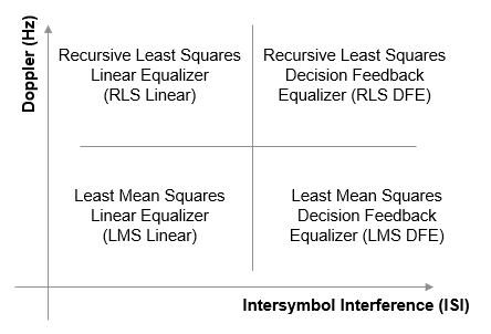
The decision feedback equalizer structure performs better than the linear equalizer structure for higher intersymbol interference.
The RLS algorithm performs better than the LMS algorithm for higher Doppler frequencies.
The LMS algorithm executes quickly, converges slowly, and its complexity grows linearly with the number of weights.
The RLS algorithm converges quickly, its complexity grows approximately as the square of the number of weights. It can be unstable when the number of weights is large.
The channels exercised for different equalizers have the following characteristics.

Initial settings for other channel impairments are the same for all equalizers. Carrier frequency offset value is set to 50 Hz. Free space path loss is set to 60 dB. Variable integer delay is set to 2 samples, which requires the equalizers to perform some timing recovery.
Deep channel fades and path loss can cause the equalizer input signal level to be much less than the desired output signal level and result in unacceptably long equalizer convergence time. The AGC block adjusts the magnitude of received signal to reduce the equalizer convergence time. You must adjust the optimal gain output power level based on the modulation scheme selected. For 16QAM, a desired output power of 10 W is used.
Training of the equalizer is performed at the beginning of the simulation.
Running the Simulation
Running the simulation computes symbol error statistics and produces these figures:
A constellation diagram of the signal after the receive filter.
A constellation diagram of the signal after adjusting gain.
A constellation diagram of the signal after equalization with signal quality measurements shown.
An equalizer error plot.
For the plots shown here, the equalizer algorithm selected is RLS Linear. Monitoring these figures, you can see that the received signal quality fluctuates as simulation time progresses.
The After Rx Filter and After AGC constellation plots show the signal before equalization. After AGC shows the impact of the channel conditions on the transmitted signal. The After Eq plot shows the signal after equalization. The signal plotted in the constellation diagram after equalization shows the variation in signal quality based on the effectiveness of the equalization process. Throughout the simulation, the signal constellations plotted before equalization deviate noticeably from a 16QAM signal constellation. The After Eq constellation improves or degrades as the equalizer error signal varies. The Eq error plotted in the Eq Error plot, indicates poor equalization at the start of the simulation. The error degrades at first then improves as the equalizer converges.


Further Exploration
Double-click the Equalizer Selector subsystem and select a different equalizer. Run the simulation to see the performance of the various equalizer options. You can use the signal logger to compare the results from this experimentation. In the model window, right-click on signal wires and select Log Selected Signals. If you have enabled signal logging, after the simulation run finishes, open the Simulation Data Inspector to view the logged signals.
At the MATLAB® command prompt, enter edit cm_ex_adaptive_eq_with_fading_init.m to open the initialization file, then modify a parameter and rerun the simulation. For example, adjust the channel characteristics (params.maxDoppler, params.pathDelays, and params.pathGains). The RLS adaptive algorithm performs better than the LMS adaptive algorithm as the maximum Doppler is increased.