looptune

Tune fixed-structure feedback loops

Syntax

[G,C,gam] = looptune(G0,C0,wc)
[G,C,gam] = looptune(G0,C0,wc,Req1,...,ReqN)
[G,C,gam] = looptune(...,options)
[G,C,gam,info] = looptune(...)


Description

[G,C,gam] = looptune(G0,C0,wc) tunes the feedback loop

to meet the following default requirements:

• Bandwidth — Gain crossover for each loop falls in the frequency interval wc

• Performance — Integral action at frequencies below wc

• Robustness — Adequate stability margins and gain roll-off at frequencies above wc

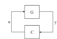
The tunable genss model C0 specifies the controller structure, parameters, and initial values. The model G0 specifies the plant. G0 can be a Numeric LTI model, or, for co-tuning the plant and controller, a tunable genss model. The sensor signals y (measurements) and actuator signals u (controls) define the boundary between plant and controller.

Note

For tuning Simulink^® models with looptune, use slTuner (Simulink Control Design) to create an interface to your Simulink model. You can then tune the control system with looptune (Simulink Control Design) for slTuner (requires Simulink Control Design™).

[G,C,gam] = looptune(G0,C0,wc,Req1,...,ReqN) tunes the feedback loop to meet additional design requirements specified in one or more tuning goal objects Req1,...,ReqN. Omit wc to use the requirements specified in Req1,...,ReqN instead of an explicit target crossover frequency and the default performance and robustness requirements.

[G,C,gam] = looptune(...,options) specifies further options, including target gain margin, target phase margin, and computational options for the tuning algorithm.

[G,C,gam,info] = looptune(...) returns a structure info with additional information about the tuned result. Use info with the loopview command to visualize tuning constraints and validate the tuned design.

Input Arguments

G0	Numeric LTI model or tunable genss model representing plant in control system to tune. The plant is the portion of your control system whose outputs are sensor signals (measurements) and whose inputs are actuator signals (controls). Use connect to build G0 from individual numeric or tunable components.
C0	Generalized LTI model representing controller. C0 specifies the controller structure, parameters, and initial values. The controller is the portion of your control system that receives sensor signals (measurements) as inputs and produces actuator signals (controls) as outputs. Use Control Design Blocks and Generalized LTI models to represent tunable components of the controller. Use connect to build C0 from individual numeric or tunable components.
wc	Vector specifying target crossover region [wcmin,wcmax]. The looptune command attempts to tune all loops in the control system so that the open-loop gain crosses 0 dB within the target crossover region. A scalar wc specifies the target crossover region [wc/2,2*wc].
Req1,...,ReqN	One or more TuningGoal objects specifying design requirements, such as TuningGoal.Tracking, TuningGoal.Gain, or TuningGoal.LoopShape.
options	Set of options for looptune algorithm, specified using looptuneOptions. See looptuneOptions for information about the available options, including target gain margin and phase margin.

Output Arguments

G	Tuned plant. If G0 is a Numeric LTI model, G is the same as G0. If G0 is a tunable genss model, G is a genss model with Control Design Blocks of the same number and types as G0. The current value of G is the tuned plant.
C	Tuned controller. C is a genss model with Control Design Blocks of the same number and types as C0. The current value of C is the tuned controller.
gam	Parameter indicating degree of success at meeting all tuning constraints. A value of gam <= 1 indicates that all requirements are satisfied. gam >> 1 indicates failure to meet at least one requirement. Use loopview to visualize the tuned result and identify the unsatisfied requirement. For best results, use the RandomStart option in looptuneOptions to obtain several minimization runs. Setting RandomStart to an integer N > 0 causes looptune to run the optimization N additional times, beginning from parameter values it chooses randomly. You can examine gam for each run to help identify an optimization result that meets your design requirements.
info	Data for validating tuning results, returned as a structure. To use the data in info, use the command loopview(G,C,info) to visualize tuning constraints and validate the tuned design. info contains the following tuning data: Di,Do Optimal input and output scalings, returned as state-space models. The scaled plant is given by Do\G*Di. Specs Design requirements that looptune constructs for its call to systune for tuning (see Algorithms), returned as a vector of TuningGoal requirement objects. Runs Detailed information about each optimization run performed by systune when called by looptune for tuning (see Algorithms), returned as a data structure. The contents of Runs are the info output of the call to systune. For information about the fields of Runs, see the info output argument description on the systune reference page.

Examples

Tune the control system of the following illustration, to achieve crossover between 0.1 and 1 rad/min.

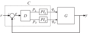
The 2-by-2 plant G is represented by:

$$G\left(s\right)=\frac{1}{75s+1}\left[\begin{array}{cc}87.8& -86.4\\ 108.2& -109.6\end{array}\right].$$

The fixed-structure controller, C, includes three components: the 2-by-2 decoupling matrix D and two PI controllers PI_L and PI_V. The signals r, y, and e are vector-valued signals of dimension 2.

Build a numeric model that represents the plant and a tunable model that represents the controller. Name all inputs and outputs as in the diagram, so that looptune knows how to interconnect the plant and controller via the control and measurement signals.

s = tf('s');
G = 1/(75*s+1)*[87.8 -86.4; 108.2 -109.6];
G.InputName = {'qL','qV'};
G.OutputName = 'y';

D = tunableGain('Decoupler',eye(2));
D.InputName = 'e';
D.OutputName = {'pL','pV'};
PI_L = tunablePID('PI_L','pi');
PI_L.InputName = 'pL';
PI_L.OutputName = 'qL';
PI_V = tunablePID('PI_V','pi'); 
PI_V.InputName = 'pV';
PI_V.OutputName = 'qV'; 
sum1 = sumblk('e = r - y',2);
C0 = connect(PI_L,PI_V,D,sum1,{'r','y'},{'qL','qV'});

wc = [0.1,1];
[G,C,gam,info] = looptune(G,C0,wc);

C is the tuned controller, in this case a genss model with the same block types as C0.

You can examine the tuned result using loopview.

Algorithms

looptune automatically converts target bandwidth, performance requirements, and additional design requirements into weighting functions that express the requirements as an H_∞ optimization problem. looptune then uses systune to optimize tunable parameters to minimize the H_∞ norm. For more information about the optimization algorithms, see [1].

looptune computes the H_∞ norm using the algorithm of [2] and structure-preserving eigensolvers from the SLICOT library. For more information about the SLICOT library, see https://github.com/SLICOT.

Alternatives

For tuning Simulink models with looptune, see slTuner (Simulink Control Design) and looptune (Simulink Control Design) (requires Simulink Control Design).

References

[1] P. Apkarian and D. Noll, "Nonsmooth H-infinity Synthesis." IEEE Transactions on Automatic Control, Vol. 51, Number 1, 2006, pp. 71–86.

[2] Bruinsma, N.A., and M. Steinbuch. "A Fast Algorithm to Compute the H_∞ Norm of a Transfer Function Matrix." Systems & Control Letters, 14, no.4 (April 1990): 287–93.

Extended Capabilities

Automatic Parallel Support

Accelerate code by automatically running computation in parallel using Parallel Computing Toolbox™.

To run in parallel, set 'UseParallel' to true using looptuneOptions.

For more information, see Speed Up Tuning with Parallel Computing Toolbox Software.

Version History

Introduced in R2016a

R2016a: Functionality moved from Robust Control Toolbox

Prior to R2016a, this functionality required a Robust Control Toolbox™ license.