append
Group models by appending their inputs and outputs
Syntax
sys = append(sys1,sys2,...,sysN)
Description
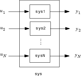
sys = append(sys1,sys2,...,sysN) appends the inputs and outputs
of the models sys1,...,sysN to form the augmented
model sys depicted below.

For systems with transfer functions
H1(s), . . . , HN(s),
the resulting system sys has the block-diagonal transfer
function
For state-space models sys1 and sys2 with data
(A1, B1, C1, D1)
and
(A2, B2, C2, D2),
append(sys1,sys2) produces the following state-space
model:
Arguments
The input arguments sys1,..., sysN can be model
objects s of any type. Regular matrices are also accepted as a representation of static
gains, but there should be at least one model in the input list. The models should be
either all continuous, or all discrete with the same sample time. When appending models
of different types, the resulting type is determined by the precedence rules (see Rules That Determine Model Type for details).
There is no limitation on the number of inputs.
Examples
Version History
Introduced before R2006a