Visualize Activations of a Deep Learning Network by Using LogoNet
This example shows how to feed an image to a convolutional neural network and display the activations of the different layers of the network. Examine the activations and discover which features the network learns by comparing areas of activation to the original image. Channels in earlier layers learn simple features like color and edges, while channels in the deeper layers learn complex features. Identifying features in this way can help you understand what the network has learned.
Logo Recognition Network
Logos assist in brand identification and recognition. Many companies incorporate their logos in advertising, documentation materials, and promotions. The logo recognition network (LogoNet) was developed in MATLAB® and can recognize 32 logos under various lighting conditions and camera motions. Because this network focuses only on recognition, you can use it in applications where localization is not required.
Prerequisites
Intel® Arria10 SoC development kit
Load Pretrained Series Network
To load the pretrained series network LogoNet, enter:
snet = getLogoNetwork;
Create Target Object
Create a target object that has a custom name for your target device and an interface to connect your target device to the host computer. Interface options are JTAG and Ethernet. To use JTAG, install Intel™ Quartus™ Prime Standard Edition 20.1. Set up the path to your installed Intel Quartus Prime executable if it is not already set up. For example, to set the toolpath, enter:
% hdlsetuptoolpath('ToolName', 'Altera Quartus II','ToolPath', 'C:\altera\20.1\quartus\bin64');To create the target object, enter:
hTarget = dlhdl.Target('Intel','Interface','JTAG');
Create Workflow Object
Create an object of the dlhdl.Workflow class. When you create the object, specify the network and the bitstream name. Specify the saved pretrained LogoNet neural network, snet, as the network. Make sure that the bitstream name matches the data type and the FPGA board that you are targeting. In this example, the target FPGA board is the Intel Arria10 SOC board. The bitstream uses a single data type.
hW = dlhdl.Workflow('network', snet, 'Bitstream', 'arria10soc_single','Target',hTarget);
Read and show an image. Save its size for future use.
im = imread('ferrari.jpg');
imshow(im)
imgSize = size(im);
imgSize = imgSize(1:2);
View Network Architecture
Analyze the network to see which layers you can view. The convolutional layers perform convolutions by using learnable parameters. The network learns to identify useful features, often including one feature per channel. The first convolutional layer has 64 channels.
analyzeNetwork(snet)
The Image Input layer specifies the input size. Before passing the image through the network, you can resize it. The network can also process larger images. If you feed the network larger images, the activations also become larger. Because the network is trained on images of size 227-by-227, it is not trained to recognize larger objects or features.
Show Activations of First Maxpool Layer
Investigate features by observing which areas in the maxpool layers activate on an image and comparing that image to the corresponding areas in the original images. Each layer of a convolutional neural network consists of many 2-D arrays called channels. Pass the image through the network and examine the output activations of the maxpool_1 layer.
act1 = hW.activations(single(im),'maxpool_1','Profiler','on');
          offset_name          offset_address     allocated_space
    _______________________    ______________    _________________

    "InputDataOffset"           "0x00000000"     "24.0 MB"
    "OutputResultOffset"        "0x01800000"     "136.0 MB"
    "SystemBufferOffset"        "0x0a000000"     "64.0 MB"
    "InstructionDataOffset"     "0x0e000000"     "8.0 MB"
    "ConvWeightDataOffset"      "0x0e800000"     "4.0 MB"
    "EndOffset"                 "0x0ec00000"     "Total: 236.0 MB"

### Programming FPGA Bitstream using JTAG...
### Programming the FPGA bitstream has been completed successfully.
### Finished writing input activations.
### Running single input activations.


              Deep Learning Processor Profiler Performance Results

                   LastLayerLatency(cycles)   LastLayerLatency(seconds)       FramesNum      Total Latency     Frames/s
                         -------------             -------------              ---------        ---------       ---------
Network                   10182024                  0.06788                       1           10182034             14.7
    conv_module           10182024                  0.06788
        conv_1             7088885                  0.04726
        maxpool_1          3093166                  0.02062
 * The clock frequency of the DL processor is: 150MHz
The activations are returned as a 3-D array, with the third dimension indexing the channel on the maxpool_1 layer. To show these activations using the imtile function, reshape the array to 4-D. The third dimension in the input to imtile represents the image color. Set the third dimension to have size 1 because the activations do not have color. The fourth dimension indexes the channel.
sz = size(act1);
act1 = reshape(act1,[sz(1) sz(2) 1 sz(3)]);
Display the activations. Each activation can take any value, so normalize the output using the mat2gray. All activations are scaled so that the minimum activation is 0 and the maximum activation is 1. Display the 96 images on an 12-by-8 grid, one for each channel in the layer.
I = imtile(mat2gray(act1),'GridSize',[12 8]);
imshow(I)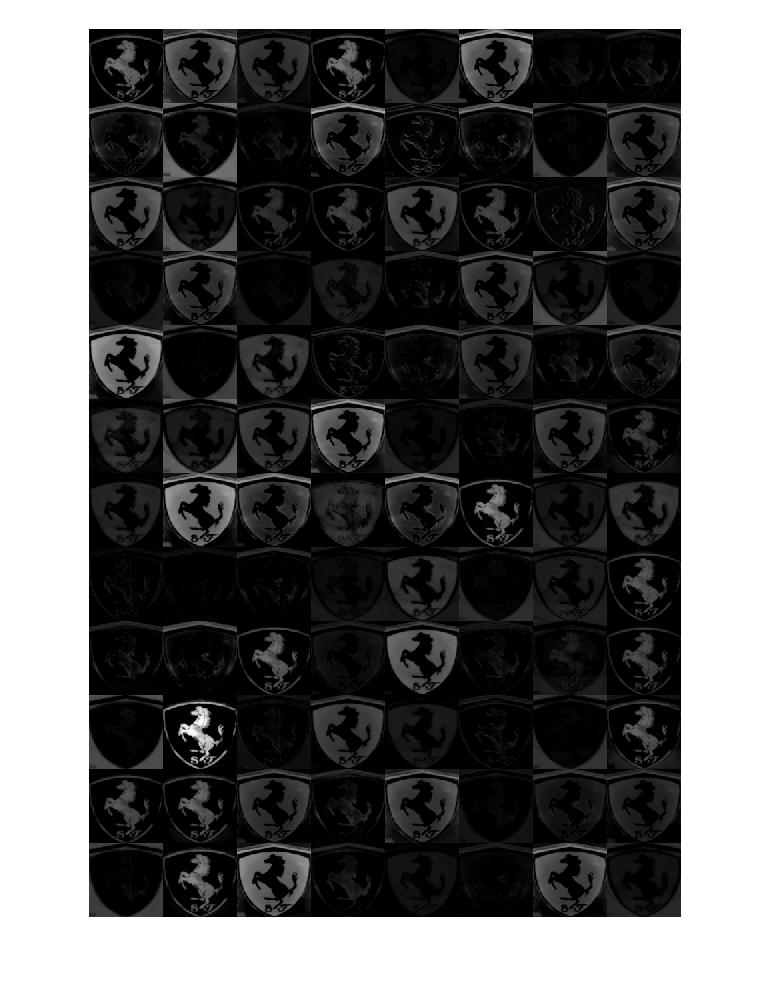
Investigate Activations in Specific Channels
Each tile in the activations grid is the output of a channel in the maxpool_1 layer. White pixels represent strong positive activations and black pixels represent strong negative activations. A channel that is mostly gray does not activate as strongly on the input image. The position of a pixel in the activation of a channel corresponds to the same position in the original image. A white pixel at a location in a channel indicates that the channel is strongly activated at that position.
Resize the activations in channel 33 to be the same size as the original image and display the activations.
act1ch33 = act1(:,:,:,22);
act1ch33 = mat2gray(act1ch33);
act1ch33 = imresize(act1ch33,imgSize);

I = imtile({im,act1ch33});
imshow(I)
Find Strongest Activation Channel
Find interesting channels by programmatically investigating channels with large activations. Find the channel that has the largest activation by using the max function, resize the channel output, and display the activations.
[maxValue,maxValueIndex] = max(max(max(act1)));
act1chMax = act1(:,:,:,maxValueIndex);
act1chMax = mat2gray(act1chMax);
act1chMax = imresize(act1chMax,imgSize);

I = imtile({im,act1chMax});
imshow(I)
Compare the strongest activation channel image to the original image. This channel activates on edges. It activates positively on light left/dark right edges and negatively on dark left/light right edges.
See Also
dlhdl.Workflow | dlhdl.Target | activations | compile | deploy | predict