Compare Deep Learning and ARMA Models for Time Series Modeling

Since R2026a

This example shows how to train and compare different models for time series modeling using the Time Series Modeler app.

Time series modeling involves predicting values based on observed data points collected over time. You can train a deep learning model for time series modeling using architectures such as recurrent neural networks, feedforward networks, or convolutional neural networks (CNNs). If you have System Identification Toolbox™, you can also train an autoregressive moving average (ARMA) model. Using the Time Series Modeler app, you can train and compare models for your task.

Import Data

When you train a time series model, there are two types of input data you can use.

• Responses: The time series you want to predict.

• Predictors: External time series that influence the responses, but which you do not want to predict. Predictors are optional, and you can train a model using only responses. These are also called exogenous predictors.

This example uses battery state-of-charge (SOC) data that contains 20 simulated observations of varying lengths, each generated for a different ambient temperature. Each observation contains the state of charge (the response) and the temperature, voltage, and current (the predictors).

load BSOC_MultipleTemperatures

Open the Time Series Modeler app.

timeSeriesModeler

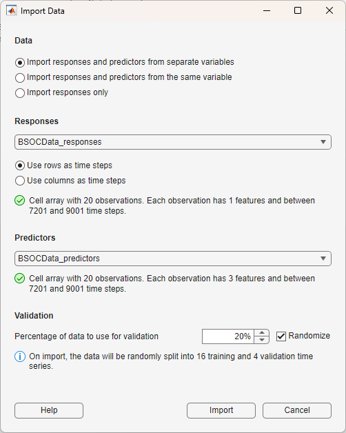
To import data into the app, click New. The Import Data dialog box opens. For the responses, select BSOCData_responses. Because this data is in "TC" (time, channel) format, meaning that the time steps are in rows and the channels are in columns, select Use rows as time steps. For the predictors, select BSOCData_predictors.

Use 20% of the data for validation and 80% for training. To randomize the data split, select Randomize.

Click Import.

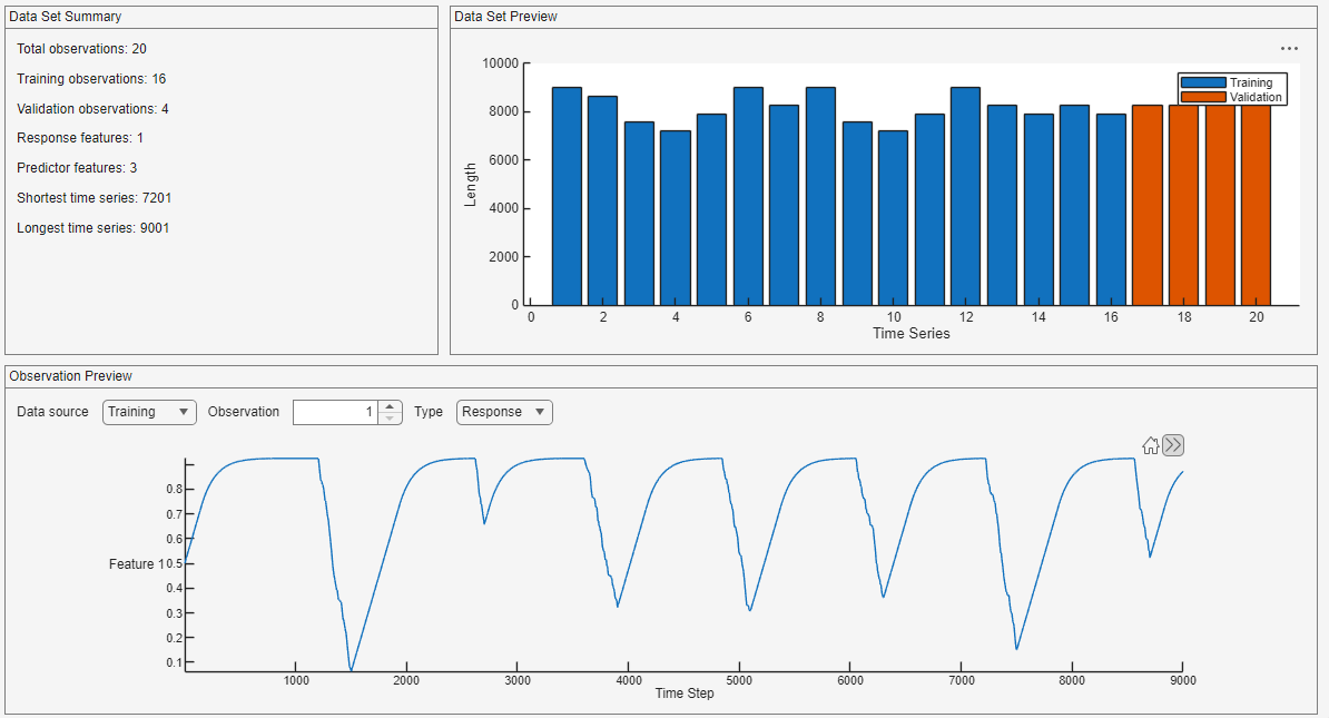
The app displays the training and validation data for both the responses and the predictors.

Train Deep Learning Models

Select a deep learning model from the Models gallery. In this example compare three models: small long short-term memory (LSTM), small multi-layer perceptron (MLP), and small CNN.

Model Name	Model Type	Description
Model 1	LSTM (Small)	LSTM networks, a type of recurrent neural network, can capture long-term dependencies in sequential data. They are suitable for time series modeling tasks where past values influence future outcomes over long periods.
Model 2	MLP (Small)	MLPs, a type of feedfoward network, are simple neural networks made up of fully connected layers. They are typically small and fast to train. MLPs do not consider the order of data and treat each input separately, which often leads to noisy predictions in time series tasks.
Model 3	CNN (Small)	CNNs use filters that process multiple time steps at once. This helps the model detect short-term patterns and reduce high-frequency noise. CNNs are effective for modeling time series with seasonal or repeating structures.

1. Click LSTM (Small). Set MaxEpochs to 1000 and then click Train.

2. Click MLP (Small). Set MaxEpochs to 1000 and then click Train.

3. Click CNN (Small). Set MaxEpochs to 1000 and then click Train.

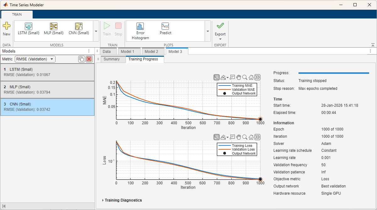
During training, the app displays training information, plots of the mean absolute error (MAE) and root mean squared error (RMSE) loss, and training diagnostics on the Training Progress tab. In the Axes toolbar above the plot, switch to the log scale to better see the change in the loss over the course of training.

To potentially improve the training values, you can experiment with changing the hyperparameters and see what effect this has on the accuracy of each model.

Compare Deep Learning Models

When choosing a deep learning model, you must trade off different attributes such as the error rate, training time, inference time, and size of the model. You might have constraints, such as that the model must be smaller than a certain size or the inference time must be below a certain threshold. You can compare different models and choose the one that best suits your task.

To easily compare the models in the app, select each model tab and drag it so that the models are side by side.

This example was run using an NVIDIA RTX A5000. Depending on your hardware, you may get different results than the example shows.

Compare Size

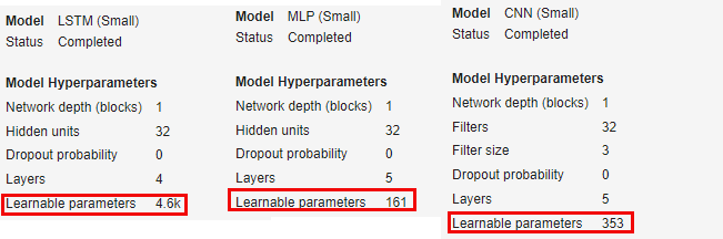
View the number of learnable parameters for each model on the Summary tab. The default LSTM architecture has many more learnable parameters than the default MLP and CNN architecture. As a result, the LSTM network takes up more space on disk if you deploy it.

Compare Training Time

When training is complete, the Training Progress tab displays the elapsed time.

Because LSTM networks capture long-term dependencies, they must track the state. The state is the long-term memory of the model and carries information across multiple time steps. This means that the LSTM model takes longer to train and has many more parameters than the default MLP and CNN models, and it cannot be trained in parallel.

In this example, the LSTM model takes over 10 minutes to train, while the MLP and CNN models both take under a minute to train.

Compare Error Rate

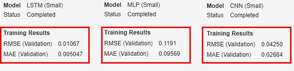
After training is complete, the Summary tab displays information about the RMSE and the MAE on the validation set. In this example, the LSTM model has the lowest error of the three models. The MLP and CNN models have similar RMSE and MAE values to one another.

Compare Predictions

For each model, click Predict. The Predict tab opens and displays the predictions of the model for each observation. Compare the predictions of each model on the first observation. You can compare the predictions side-by-side by dragging the Predict windows.

The LSTM (Model 1) matches the true values well. The predictions of the MLP (Model 2) are much noisier. The CNN (Model 3) matches the general pattern of the true values and is less noisy than the MLP, but noisier than the LSTM.

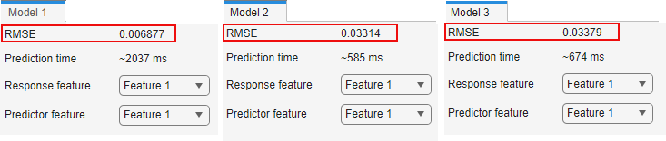
The Predict tab shows, you can see the RMSE for the selected observation. The LSTM model fits the true values much better than the MLP and CNN models.

Compare Inference Time

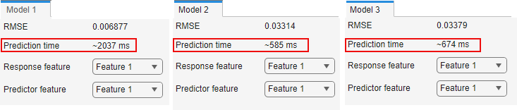
In the Predict tab, you can also see the estimated prediction time, also called inference time, for each observation. The prediction time will vary even with the same model on the same observation. On the NVIDIA RTX A5000 that was used to run this example, the LSTM model takes much longer to predict than the MLP or CNN models.

Summary

Overall, the LSTM model achieves better inference performance than the other two models, at the cost of being bigger, slower to train, and slower to perform inference. The MLP model is the smallest and quickest, but has a higher error rate than the LSTM model. To further optimize these models requires empirical analysis. To explore different model and training configurations by running experiments, you can use the Experiment Manager app.

Export Deep Learning Model

Once you are happy with the trained model, you can export it and use it on new test data. To export the model and generate code to predict new values for test data, click Export.

Train ARMA Model

If you have System Identification Toolbox, you can also train and export an ARMA model. In the app, from the Models gallery, click ARMA Model. On the Summary tab, keep the default values for all the model structure and training options. Click Train. ARMA models are smaller and faster to train when compared to deep learning models. So, instead of training a single ARMA model, the app trains multiple models and selects the best models to display.

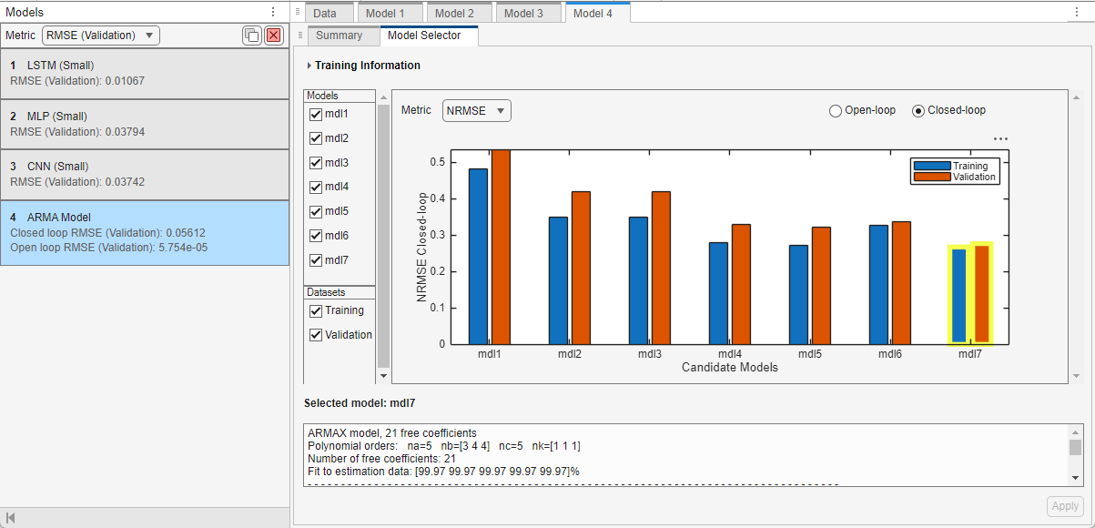
After training, a plot displaying a set of candidate models and their respective NRMSE values appears on the Model Selector tab. At the top of the plot, in the Metric menu, you can choose other quality metrics that you want the plot to display. The available quality metrics are RMSE, NRMSE, MAE, AIC, and BIC. If you select Metric as RMSE, NRMSE, or MAE, you can select Open-loop or Closed-loop at the top right of the plot to display the respective plots. Selecting Open-loop is equivalent to specifying the prediction horizon input argument for the predict (System Identification Toolbox) command as 1, that is, performing a one-step-ahead prediction of the ARMA model. Selecting Closed-loop is equivalent to specifying the prediction horizon input argument for the predict (System Identification Toolbox) command as Inf, that is, performing a simulation of the ARMA model.

To the left of the plot, in the Models section, you can choose all the models that you want to display. In the Datasets section, you can choose to display the Training dataset, Validation dataset, or both.

The qualities of the candidate models change based on the metric type and metric setting you choose. For a chosen metric, the candidate model with a lower metric value is better. Some metrics such as AIC and BIC naturally protect against overfitting by penalizing the model complexity.

The minimum values for the metrics provide an optimal tradeoff between the model performance and model complexity. For a selected model, you can see the model complexity information, that is, the number of free coefficients in the model, in the text box below the plot. You can use this information to perform a manual tradeoff between the model quality, as shown by the MAE, NRMSE, or RMSE metrics, and the corresponding complexity.

The plot automatically highlights and selects the model with the lowest NRMSE value on training data in the closed-loop metric setting. You can select a different model by clicking the model in the plot or selecting it in the Select model list.

For this example, to finalize the model selected by the app and complete the training process, click Apply.

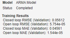
View the Training Results on the Summary tab of the app.

To predict values for the training and validation data using the selected model, on the Train tab, click Predict. Set the Prediction type, Data source, Response feature, and Predictor feature to view the corresponding response vs prediction plots. For this example, set the Prediction type as Closed loop and Data source as Validation. You can see that the predictions of the trained model match the true values well.

To export the trained model and generate code to predict new values for test data, on the Train tab, click Export.

For more information on ARMA model training, see Estimate ARMA Model Using Time Series Modeler app (System Identification Toolbox).