Denoise ECG Signals Using Deep Learning

Since R2026a

This example shows how to interactively train deep neural networks to remove noise from heartbeat electrocardiogram (ECG) signals using the Time Series Modeler app. You can train a deep neural network to map noisy signals to clean ones and achieve a better signal-to-noise ratio than you could with classical techniques like moving averages. You can use the Time Series Modeler app to build, train, and compare models for time series forecasting.

By default, the app trains the network using a GPU if one is available and if you have Parallel Computing Toolbox™.

Load and Prepare Data

This example uses the PhysioNet ECG-ID database [1] [2], which has 310 ECG records from 90 subjects. Each record contains a raw, noisy ECG signal and a manually-filtered, clean, ground truth version of the same signal.

Save the data set to a local folder or download the data using the following code.

datasetFolder = fullfile(tempdir,"ecg-id-database-1.0.0");
if ~isfolder(datasetFolder)
    loc = websave(tempdir,"https://physionet.org/static/published-projects/ecgiddb/ecg-id-database-1.0.0.zip");
    unzip(loc,tempdir);
end

To reads the ECG data from the file, use the helperReadSignalData helper function, which is provided at the end of this example. Create a signalDatastore (Signal Processing Toolbox) object to manage the data.

sds = signalDatastore(datasetFolder, ...
    IncludeSubfolders = true, ...
    FileExtensions = ".dat", ...
    ReadFcn = @helperReadSignalData);

Select data randomly from 10 different subjects as the test set.

rng("default")
subjectIds = unique(extract(sds.Files,"Person_"+digitsPattern));
testSubjects = contains(sds.Files,subjectIds(randperm(numel(subjectIds),10)));
testDs = subset(sds,testSubjects);

trainAndValDs = subset(sds,~testSubjects);
trainAndValDs = shuffle(trainAndValDs);

Read the train and test data into memory. Then, convert the cell array into separate predictor and response cell arrays. The predictors are the noisy ECG signals, and the responses are the corresponding clean signals.

data = trainAndValDs.readall();
predictors = {};
responses = {};
for i=1:size(data,1)
    predictors{i,1} = data{i}{1};
    responses{i,1} = data{i}{2};
end

Rescale ECG Traces

The response data contains some outliers, which are larger than the typical response value. This destabilizes training. To avoid this, rescale each ECG trace separately, so that all traces have the same scale.

for i=1:size(data,1)
    predictors{i,1} = rescale(predictors{i,1});
    responses{i,1} = rescale(responses{i,1});
end

Split Data into Shorter Windows

Each file has 10,000 time steps. For easier processing by deep neural networks, divide each file into shorter windows of 400 time steps. This division lets you build networks with fewer learnable parameters, makes the memory manageable for the neural networks, and speeds up training. This division also moves the data from the time dimension to the batch dimension. In the batch dimension, the data is processed in parallel. As a result, the network sees more data at any given time during training, further speeding up training. The Time Series Modeler app can split a single time series into windows but in this example, the data has multiple time series, so you must manually split the data.

predictorsCell = {};
responsesCell = {};
windowLength = 400;
for i=1:length(predictors)
    numWindows = floor(length(predictors{i})/windowLength);
    for j=1:numWindows
        predictorsCell{end+1,1} = predictors{i}(1+(j-1)*windowLength:j*windowLength);
        responsesCell{end+1,1} = responses{i}(1+(j-1)*windowLength:j*windowLength);
    end
end

Train Deep Neural Networks in Time Series Modeler

Open the Time Series Modeler app.

timeSeriesModeler

To import the predictors and responses into the app, click the New button on the toolstrip. The Import Data dialog box opens.

In the Import Data dialog box, select Import responses and predictors from separate variable. Under Responses, select responsesCell and under Predictors, select predictorsCell. To use the last 20% of the time series as validation data, keep the default value of 20% in the Percentage of data to use for validation box. Click Import.

On the Data tab, in the Observation Preview pane, examine some of the observations you imported. For each observation you examine, in the Observation Preview pane, switch the Type between Predictor and Response to verify that each response is a clean version of the corresponding predictor.

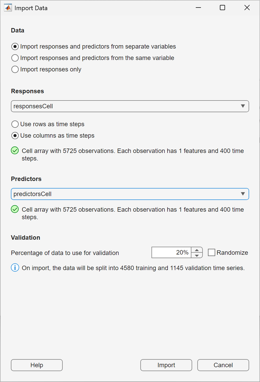
Train Multilayer Perceptron

A multilayer perceptron (MLP) is a simple neural network with only fully connected layers. It does not model temporal history and simply maps inputs to outputs.

On the toolstrip, in the Models gallery, select MLP (Small). The Summary tab opens. Keep the default settings in the Summary tab. On the toolstrip, click Train. Training on the entire dataset takes a long time. Since the MLP does not use temporal history and is unlikely to perform well, stop training after a minute by clicking Stop.

Click Predict.

Notice that the MLP is susceptible to high-frequency noise and cannot capture the peaks of the time series.

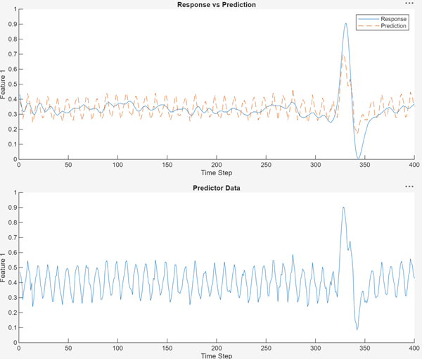
Train Convolutional Neural Network

A 1-D convolutional neural network (1-D CNN) is more effective than an MLP at removing high-frequency noise because its convolutional filters operate over multiple time steps.

To create a 1-D CNN, select CNN (small). In the Summary tab, set the Filter size to seven. This allows the network to learn to denoise over about seven time steps. Set the Network depth (blocks) to two. Train the network and stop training after a minute.

The 1-D CNN is more effective than the MLP at removing noise from data and capturing the peak of the ECG trace.

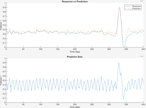
Train Recurrent Neural Network

Finally, train a long short-term memory (LSTM) neural network, which is a type of recurrent neural network. LSTMs have long memory but can be affected by high-frequency noise. Select LSTM (Small). Train the network and stop training after a minute.

This network smoothly captures the peak but still has some high-frequency noise.

Compare to Classical Denoising Techniques

This section compares the denoising performance of the deep neural network to that of a classical algorithm. The deep neural network performs better at denoising and gives a better signal-to-noise ratio. To export the trained 1-D CNN model to the workspace, click Export to Workspace. The app assigns the model to the variable trainedModel_1. Store the trained network as net.

load trainedModel_1.mat
net = trainedModel_1.TrainedModel;

Extract the validation predictors and responses.

noisyECGs = predictorsCell(5601:end);
cleanECGs = responsesCell(5601:end);

Use the CNN to denoise the noisy ECG validation data.

denoisedCNN = {};
for i=1:length(noisyECGs)
    denoisedCNN{i} = predict(net, noisyECGs{i}, InputDataFormats="CTB");
end

Perform equivalent denoising using a classical technique. For this example, use the smoothdata with a moving-mean smoothing method and a window of nine time steps. The function removes high‑frequency noise from an ECG signal by using a low-pass finite impulse response (FIR) filter to preserve only the relevant low‑frequency cardiac components.

denoisedClassical = {};
for i=1:length(noisyECGs)
    denoisedClassical{i} = smoothdata(noisyECGs{i}, "movmean", 9);
end

Compute the signal-to-noise ratio (SNR) for each approach using the snr (Signal Processing Toolbox) function: no denoising, classical denoising, and denoising with the 1-D CNN. A higher SNR indicates more effective denoising.

for i=1:size(noisyECGs, 1)
    snrNoisy(i,1) = snr(cleanECGs{i}, cleanECGs{i} - noisyECGs{i});
    snrClassical(i,1) = snr(cleanECGs{i}, cleanECGs{i} - denoisedClassical{i});
    snrCNN(i,1) = snr(cleanECGs{i}, cleanECGs{i} - denoisedCNN{i});
end

Plot the bar chart of the SNRs for each technique.

snrs = [snrNoisy, snrClassical, snrCNN];
bar(mean(snrs))
xticklabels(["Noisy", "Classical", "1-D CNN"])
ylabel("SNR")

The chart shows that CNN has a better SNR than the classical method. This is because the CNN preserves the peak’s height and shape, while the classical method smooths it out.

Plot a few ECG signals and their denoised signals to compare the results.

t = tiledlayout(2, 2)

t = 
  TiledChartLayout with properties:

    TileArrangement: 'fixed'
           GridSize: [2 2]
            Padding: 'loose'
        TileSpacing: 'loose'

  Show all properties

for i=1:4
    ax = nexttile(t);
    hold on
    plot(ax, noisyECGs{i})
    plot(ax, denoisedClassical{i})
    plot(ax, denoisedCNN{i})
end
legend(ax, ["Noisy", "Classical", "CNN"])

Helper Functions

The helperReadSignalData function reads PhysioNet ECG data from a file.

function [dataOut,infoOut] = helperReadSignalData(filename)
fid = fopen(filename,"r");
% 1st row : raw data, 2nd row : filtered data
data = fread(fid,[2 Inf],"int16=>single");
fclose(fid);
fid = fopen(replace(filename,".dat",".hea"),"r");
header = textscan(fid,"%s%d%d%d",2,"Delimiter"," ");
fclose(fid);
gain = single(header{3}(2));
dataOut{1} = data(1,:)/gain; % noisy, raw data
dataOut{2} = data(2,:)/gain; % filtered, clean data
infoOut.SampleRate = header{3}(1);
end

References

[1] Lugovaya, Tatiana. 2005. "Biometric Human Identification Based on Electrocardiogram." Master's thesis, Saint Petersburg Electrotechnical University.

[2] Goldberger, Ary L., Luis A. N. Amaral, Leon Glass, Jeffrey M. Hausdorff, Plamen Ch. Ivanov, Roger G. Mark, Joseph E. Mietus, George B. Moody, Chung-Kang Peng, and H. Eugene Stanley. “PhysioBank, PhysioToolkit, and PhysioNet.” Circulation 101, no. 23 (June 13, 2000): e215–20. https://doi.org/10.1161/01.CIR.101.23.e215.