Reconstruction Through Two-Channel Filter Banks

This example shows how to design perfect reconstruction two-channel filter banks, also known as the Quadrature Mirror Filter (QMF) banks. The QMF banks use power complementary filters.

There are several digital signal processing applications in which signals are first split into low frequency and high frequency subbands, and later these subbands are combined to reconstruct the original signal. One such application is subband coding (SBC).

First simulate the perfect reconstruction process by filtering a signal made up of scaled and time shifted impulses. Then plot the input, output, and error signals along with the magnitude spectrum of the transfer function of the complete system. The effectiveness of the perfect reconstruction is shown through the filter bank described in this example.

Perfect Reconstruction

A system is said to achieve perfect reconstruction when the output of the system is equal to the input signal or a delayed version of the same. Below is a block diagram of a perfect reconstruction process which uses ideal filters to separate the signal into its low frequency and high frequency components, and to recover the signal completely. The perfect reconstruction process requires four filters, two lowpass filters (${\mathit{H}}_0$and ${\mathit{G}}_0$) and two highpass filters (${\mathit{H}}_1$and ${\mathit{G}}_1$). In addition, the process requires a downsampler and an upsampler between the two lowpass and the two highpass filters. Since the analysis filters have unit gain, the synthesis filters compensate for the preceding upsamplers by having a gain of 2.

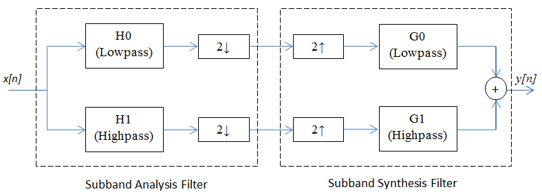
Perfect Reconstruction Two-Channel Filter Bank

The DSP System Toolbox™ provides a specialized function called firpr2chfb to design the four filters required to implement an FIR perfect reconstruction two-channel filter bank. The firpr2chfb function designs the four FIR filters for the analysis (${\mathit{H}}_0$and ${\mathit{H}}_1$) and synthesis (${\mathit{G}}_0$and ${\mathit{G}}_1$) sections of a two-channel perfect reconstruction filter bank. The design corresponds to orthogonal filter banks known as power-symmetric filter banks, which are required in order to achieve the perfect reconstruction.

Design a filter bank with filters of order 99, passband edges of the lowpass and highpass filters at 0.45 and 0.55, respectively:

N = 99;
[LPAnalysis, HPAnalysis, LPSynthsis, HPSynthesis] = firpr2chfb(N, 0.45);

The magnitude response of these filters is plotted below:

FA = filterAnalyzer(LPAnalysis,1, HPAnalysis,1, LPSynthsis,1, HPSynthesis,1);
setLegendStrings(FA,["Hlp Lowpass Decimator","Hhp Highpass Decimator",...
    "Glp Lowpass Interpolator","Ghp Highpass Interpolator"]);

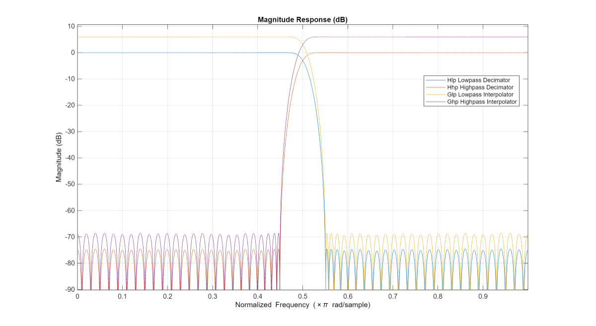
Note that the analysis path consists of a filter followed by a downsampler, which is a decimator, and the synthesis path consists of an upsampler followed by a filter, which is an interpolator. The DSP System Toolbox provides dsp.SubbandAnalysisFilter and dsp.SubbandSynthesisFilter objects to implement the analysis portion and the synthesis portion of the filter bank, respectively.

% Analysis section
analysisFilter = dsp.SubbandAnalysisFilter(LPAnalysis, HPAnalysis);
% Synthesis section
synthFilter = dsp.SubbandSynthesisFilter(LPSynthsis, HPSynthesis);

For the sake of an example, let p[n] denote the signal

$$\mathit{p}\left[\mathit{n}\right]=\delta \left[\mathit{n}\right]+\delta \left[\mathit{n}-1\right]+\delta \left[\mathit{n}-2\right]$$

and let the signal x[n] be defined by

$$\mathit{x}\left[\mathit{n}\right]=\mathit{p}\left[\mathit{n}\right]+2\mathit{p}\left[\mathit{n}-8\right]+3\mathit{p}\left[\mathit{n}-16\right]+4\mathit{p}\left[\mathit{n}-24\right]+3\mathit{p}\left[\mathit{n}-32\right]+2\mathit{p}\left[\mathit{n}-40\right]+\mathit{p}\left[\mathit{n}-48\right]$$

Note: Since MATLAB® uses one-based indexing, delta[n] = 1 when n = 1.

x = zeros(50,1);
x(1:3)   = 1;
x(8:10)  = 2;
x(16:18) = 3;
x(24:26) = 4;
x(32:34) = 3;
x(40:42) = 2;
x(48:50) = 1;
sigsource = dsp.SignalSource(SignalEndAction="Cyclic repetition",...
                                SamplesPerFrame=50);
sigsource.Signal = x;

To view the results of the simulation, we need four scopes:

1. To compare the input signal with the reconstructed output.

2. To measure the error between the input signal and the reconstructed output

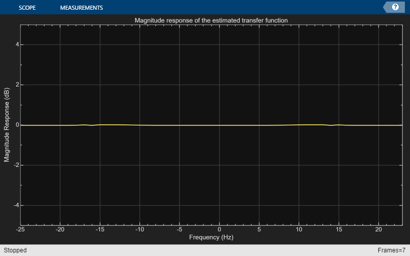
3. To plot the magnitude response of the overall system.

4. To plot the phase response of the overall system.

% Scope to compare input signal with reconstructed output
sigcompare = dsp.ArrayPlot(NumInputPorts=2, ShowLegend=true,...
                            Title="Input and reconstructed signals",...
                            ChannelNames=["Input signal","Reconstructed signal"]);

% Scope to plot the RMS error between the input and reconstructed signals
errorPlot = timescope(Title="RMS Error",SampleRate=1, ...
                        TimeUnits="seconds", YLimits=[-0.5 2],...
                        TimeSpanSource="property",TimeSpan=100,...
                        TimeSpanOverrunAction="scroll");

% To calculate the transfer function of the cascade of Analysis and
% Synthesis subband filters
tfestimate = dsp.TransferFunctionEstimator(FrequencyRange="centered",...
                                            SpectralAverages=50);
% Scope to plot the magnitude response of the estimated transfer function
magplot = dsp.ArrayPlot(PlotType="Line", ...
    YLabel="Magnitude Response (dB)",...
    Title="Magnitude response of the estimated transfer function",...
    XOffset=-25, XLabel="Frequency (Hz)",...
    YLimits=[-5 5]);
% Scope to plot the phase response of the estimated transfer function
phaseplot = dsp.ArrayPlot(PlotType="Line", ...
    YLabel="Phase Response (degrees)",...
    Title="Phase response of the estimated transfer function",...
    XOffset=-25, XLabel="Frequency (Hz)",...
    YLimits=[-180 180]);

Simulation of Perfect Reconstruction

Pass the input signal through the subband filters and reconstruct the output. Plot the results on the scopes.

for i = 1:100
    % Use the same signal as input in each iteration.
    input = sigsource();
    % Analysis
    [hi, lo] = analysisFilter(input);
    % Synthesis
    reconstructed = synthFilter(hi, lo);

    % Compensate for the delay caused by the filters and compare the
    % signals. Since input signal is periodic, compare the current
    % frames of input and output signals.
    sigcompare(input(2:end), reconstructed(1:end-1));

    % Plot error between signals
    err = rms(input(2:end) - reconstructed(1:end-1));
    errorPlot(err);

    % Estimate transfer function of cascade
    Txy = tfestimate(input(2:end), reconstructed(1:end-1));
    magplot(20*log10(abs(Txy)));
    phaseplot(angle(Txy)*180/pi);
end

release(errorPlot);

release(magplot);

release(phaseplot);

Perfect Reconstruction Output Analysis

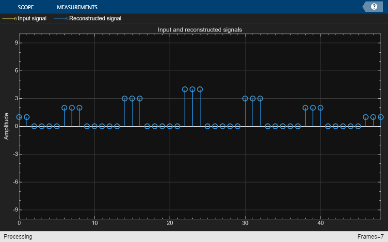
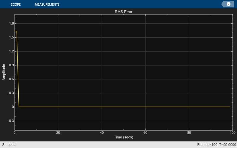
The first two plots show that the two-channel filter bank perfectly reconstructs the original signal x[n]. The initial error in the second plot is due to delay in the filters. The third and the fourth plots show that the overall system has a magniude response of 0 dB and phase response of 0°, thereby preserving the frequency characteristics of the signal.

Related Topics

• Overview of Filter Banks
• Two-Channel Filter Bank Using Halfband Decimators and Halfband Interpolators
• Multilevel Filter Banks