optSensByBatesNI

Option price or sensitivities by Bates model using numerical integration

Syntax

PriceSens = optSensByBatesNI(Rate,AssetPrice,Settle,Maturity,OptSpec,Strike,V0,ThetaV,Kappa,SigmaV,RhoSV,MeanJ,JumpVol,JumpFreq)

PriceSens = optSensByBatesNI(___,Name,Value)

Description

PriceSens = optSensByBatesNI(Rate,AssetPrice,Settle,Maturity,OptSpec,Strike,V0,ThetaV,Kappa,SigmaV,RhoSV,MeanJ,JumpVol,JumpFreq) computes vanilla European option price and sensitivities by Bates model, using numerical integration methods.

PriceSens = optSensByBatesNI(___,Name,Value) adds optional name-value pair arguments.

Examples

Workflow for Plotting an Option Sensitivity Surface Using the Bates Model

optSensByBatesNI uses numerical integration to compute option sensitivities and then to plot option sensitivity surfaces.

Define Option Variables and Bates Model Parameters

AssetPrice = 80;
Rate = 0.03;
DividendYield = 0.02;
OptSpec = 'call';

V0 = 0.04;
ThetaV = 0.05;
Kappa = 1.0;
SigmaV = 0.2;
RhoSV = -0.7;
MeanJ = 0.02;
JumpVol = 0.08;
JumpFreq = 2;

Compute the Option Sensitivity for a Single Strike

Settle = datenum('29-Jun-2017');
Maturity = datemnth(Settle, 6);
Strike = 80; 

Delta = optSensByBatesNI(Rate, AssetPrice, Settle, Maturity, OptSpec, Strike, ...
    V0, ThetaV, Kappa, SigmaV, RhoSV, MeanJ, JumpVol, JumpFreq, ...
    'DividendYield', DividendYield, 'OutSpec', "delta")

Delta = 0.5630

Compute the Option Sensitivities for a Vector of Strikes

The Strike input can be a vector.

Settle = datenum('29-Jun-2017');
Maturity = datemnth(Settle, 6);
Strike = (76:2:84)';

Delta = optSensByBatesNI(Rate, AssetPrice, Settle, Maturity, OptSpec, Strike, ...
    V0, ThetaV, Kappa, SigmaV, RhoSV, MeanJ, JumpVol, JumpFreq, ...
    'DividendYield', DividendYield, 'OutSpec', "delta")

Delta = 5×1

    0.6807
    0.6234
    0.5630
    0.5011
    0.4392

Compute the Option Sensitivities for a Vector of Strikes and a Vector of Dates of the Same Lengths

Use the Strike input to specify the strikes. Also, the Maturity input can be a vector, but it must match the length of the Strike vector if the ExpandOutput name-value pair argument is not set to "true".

Settle = datenum('29-Jun-2017');
Maturity = datemnth(Settle, [12 18 24 30 36]); % Five maturities
Strike = [76 78 80 82 84]'; % Five strikes

Delta  = optSensByBatesNI(Rate, AssetPrice, Settle, Maturity, OptSpec, Strike, ...
    V0, ThetaV, Kappa, SigmaV, RhoSV, MeanJ, JumpVol, JumpFreq, ...
    'DividendYield', DividendYield, 'OutSpec', "delta") % Five values in vector output

Delta = 5×1

    0.6625
    0.6232
    0.5958
    0.5748
    0.5577

Expand the Output for a Surface

Set the ExpandOutput name-value pair argument to "true" to expand the output into a NStrikes-by-NMaturities matrix. In this case, it is a square matrix.

Delta  = optSensByBatesNI(Rate, AssetPrice, Settle, Maturity, OptSpec, Strike, ...
    V0, ThetaV, Kappa, SigmaV, RhoSV, MeanJ, JumpVol, JumpFreq, ...
    'DividendYield', DividendYield, 'OutSpec', "delta", ...
    'ExpandOutput', true) % (5 x 5) matrix output

Delta = 5×5

    0.6625    0.6556    0.6515    0.6483    0.6455
    0.6222    0.6232    0.6239    0.6241    0.6238
    0.5805    0.5900    0.5958    0.5996    0.6019
    0.5381    0.5564    0.5674    0.5748    0.5798
    0.4954    0.5225    0.5389    0.5499    0.5577

Compute the Option Sensitivities for a Vector of Strikes and a Vector of Dates of Different Lengths

When ExpandOutput is "true", NStrikes do not have to match NMaturities. That is, the output NStrikes -by- NMaturities matrix can be rectangular.

Settle = datenum('29-Jun-2017');
Maturity = datemnth(Settle, 12*(0.5:0.5:3)'); % Six maturities
Strike = (76:2:84)'; % Five strikes

Delta  = optSensByBatesNI(Rate, AssetPrice, Settle, Maturity, OptSpec, Strike, ...
    V0, ThetaV, Kappa, SigmaV, RhoSV, MeanJ, JumpVol, JumpFreq, ...
    'DividendYield', DividendYield, 'OutSpec', "delta", ...
    'ExpandOutput', true)  % (5 x 6) matrix output

Delta = 5×6

    0.6807    0.6625    0.6556    0.6515    0.6483    0.6455
    0.6234    0.6222    0.6232    0.6239    0.6241    0.6238
    0.5630    0.5805    0.5900    0.5958    0.5996    0.6019
    0.5011    0.5381    0.5564    0.5674    0.5748    0.5798
    0.4392    0.4954    0.5225    0.5389    0.5499    0.5577

Compute the Option Sensitivities for a Vector of Strikes and a Vector of Asset Prices

When ExpandOutput is "true", the output can also be a NStrikes-by-NAssetPrices rectangular matrix by accepting a vector of asset prices.

Settle = datenum('29-Jun-2017');
Maturity = datemnth(Settle, 12); % Single maturity
ManyAssetPrices = [70 75 80 85]; % Four asset prices
Strike = (76:2:84)'; % Five strikes

Delta  = optSensByBatesNI(Rate, ManyAssetPrices, Settle, Maturity, OptSpec, Strike, ...
    V0, ThetaV, Kappa, SigmaV, RhoSV, MeanJ, JumpVol, JumpFreq, ...
    'DividendYield', DividendYield, 'OutSpec', "delta", ...
    'ExpandOutput', true) % (5 x 4) matrix output

Delta = 5×4

    0.4350    0.5579    0.6625    0.7457
    0.3881    0.5124    0.6222    0.7120
    0.3432    0.4670    0.5805    0.6763
    0.3010    0.4223    0.5381    0.6390
    0.2619    0.3789    0.4954    0.6002

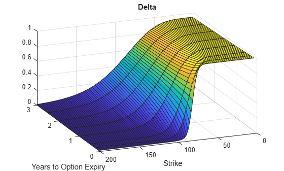
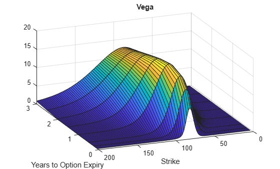
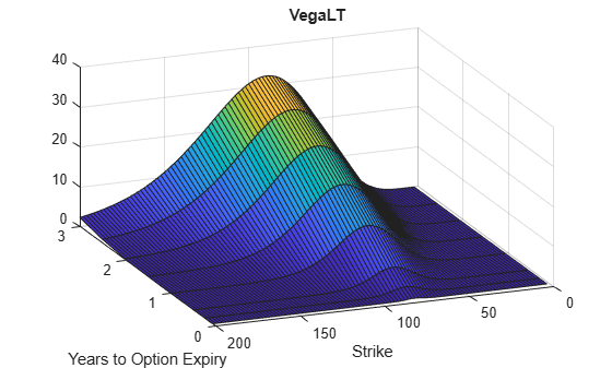
Plot Option Sensitivity Surfaces

The Strike and Maturity inputs can be vectors. Set ExpandOutput to "true" to output the surfaces as NStrikes-by-NMaturities matrices.

Settle = datenum('29-Jun-2017');
Maturity = datemnth(Settle, 12*[1/12 0.25 (0.5:0.5:3)]');
Times = yearfrac(Settle, Maturity);
Strike = (2:2:200)';

[Delta, Gamma, Rho, Theta, Vega, VegaLT] = optSensByBatesNI(...
    Rate, AssetPrice, Settle, Maturity, OptSpec, Strike, V0, ThetaV, Kappa, ...
    SigmaV, RhoSV, MeanJ, JumpVol, JumpFreq, 'DividendYield', DividendYield, ...
    'OutSpec', ["delta", "gamma", "rho", "theta", "vega", "vegalt"], ...
    'ExpandOutput', true);

[X,Y] = meshgrid(Times,Strike);

figure;
surf(X,Y,Delta);
title('Delta');
xlabel('Years to Option Expiry');
ylabel('Strike');
view(-112,34);
xlim([0 Times(end)]);

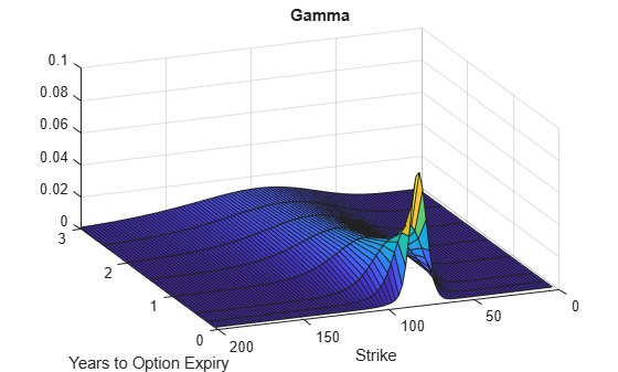
figure;
surf(X,Y,Gamma)
title('Gamma')
xlabel('Years to Option Expiry')
ylabel('Strike')
view(-112,34);
xlim([0 Times(end)]);

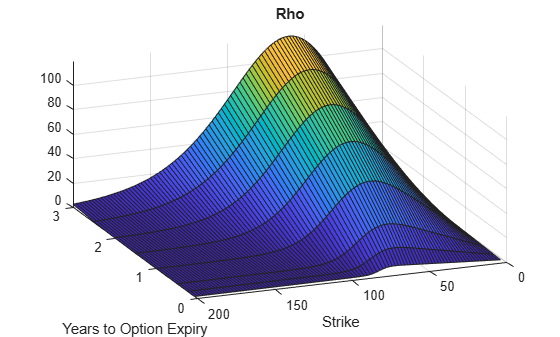
figure;
surf(X,Y,Rho)
title('Rho')
xlabel('Years to Option Expiry')
ylabel('Strike')
view(-112,34);
xlim([0 Times(end)]);

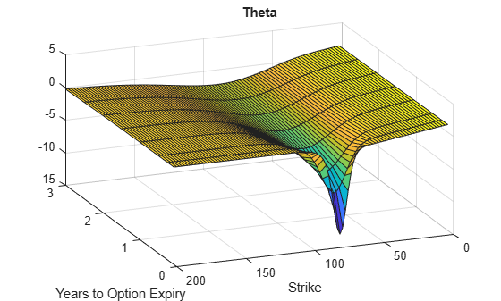
figure;
surf(X,Y,Theta)
title('Theta')
xlabel('Years to Option Expiry')
ylabel('Strike')
view(-112,34);
xlim([0 Times(end)]);

figure;
surf(X,Y,Vega)
title('Vega')
xlabel('Years to Option Expiry')
ylabel('Strike')
view(-112,34);
xlim([0 Times(end)]);

figure;
surf(X,Y,VegaLT)
title('VegaLT')
xlabel('Years to Option Expiry')
ylabel('Strike')
view(-112,34);
xlim([0 Times(end)]);

Input Arguments

Rate — Continuously compounded risk-free interest rate

decimal

Continuously compounded risk-free interest rate, specified as a scalar decimal value.

Data Types: double

AssetPrice — Current underlying asset price

numeric

Current underlying asset price, specified as numeric value using a scalar or a NINST-by-1 or NColumns-by-1 vector.

For more information on the proper dimensions for AssetPrice, see the name-value pair argument ExpandOutput.

Data Types: double

Settle — Option settlement date

serial date number | date character vector | datetime | string array

Option settlement date, specified as a NINST-by-1 or NColumns-by-1 vector using serial date numbers, date character vectors, datetime arrays, or string arrays. The Settle date must be before the Maturity date.

For more information on the proper dimensions for Settle, see the name-value pair argument ExpandOutput.

Data Types: double | char | datetime | string

Maturity — Option maturity date

serial date number | date character vector | datetime | string array

Option maturity date, specified as a NINST-by-1 or NColumns-by-1 vector using serial date numbers, date character vectors, datetime arrays, or string arrays.

For more information on the proper dimensions for Maturity, see the name-value pair argument ExpandOutput.

Data Types: double | char | datetime | string

OptSpec — Definition of option

cell array of character vector with values 'call' or 'put' | string array with values "call" or "put"

Definition of the option, specified as a NINST-by-1 or NColumns-by-1 vector using a cell array of character vectors or string arrays with values 'call' or 'put'.

For more information on the proper dimensions for OptSpec, see the name-value pair argument ExpandOutput.

Data Types: cell | string

Strike — Option strike price value

numeric

Option strike price value, specified as a NINST-by-1, NRows-by-1, NRows-by-NColumns vector of strike prices.

For more information on the proper dimensions for Strike, see the name-value pair argument ExpandOutput.

Data Types: double

V0 — Initial variance of underlying asset

numeric

Initial variance of the underling asset, specified as a scalar numeric value.

Data Types: double

ThetaV — Long-term variance of underlying asset

numeric

Long-term variance of the underling asset, specified as a scalar numeric value.

Data Types: double

Kappa — Mean revision speed for the variance of underlying asset

numeric

Mean revision speed for the underling asset, specified as a scalar numeric value.

Data Types: double

SigmaV — Volatility of the variance of underlying asset

numeric

Volatility of the variance of the underling asset, specified as a scalar numeric value.

Data Types: double

RhoSV — Correlation between Weiner processes for underlying asset and its variance

numeric

Correlation between the Weiner processes for the underlying asset and its variance, specified as a scalar numeric value.

Data Types: double

MeanJ — Mean of the random percentage jump size

decimal

Mean of the random percentage jump size (J), specified as a scalar decimal value where log(1+J) is normally distributed with mean (log(1+MeanJ)-0.5*JumpVol^2) and the standard deviation JumpVol.

Data Types: double

JumpVol — Standard deviation of log(1+J)

decimal

Standard deviation of log(1+J) where J is the random percentage jump size, specified as a scalar decimal value.

Data Types: double

JumpFreq — Annual frequency of Poisson jump process

numeric

Annual frequency of Poisson jump process, specified as a scalar numeric value.

Data Types: double

Name-Value Arguments

Specify optional comma-separated pairs of Name,Value arguments. Name is the argument name and Value is the corresponding value. Name must appear inside quotes. You can specify several name and value pair arguments in any order as Name1,Value1,...,NameN,ValueN.

Example: PriceSens = optSensByBatesNI(Rate,AssetPrice,Settle,Maturity, OptSpec,Strike,V0,ThetaV,Kappa,SigmaV,RhoSV,MeanJ,JumpVol,JumpFreq,'Basis',7)

Basis — Day-count basis of instrument

0 (default) | numeric values: 0,1, 2, 3, 4, 6, 7, 8, 9, 10, 11, 12, 13

Day-count of the instrument, specified as the comma-separated pair consisting of 'Basis' and a scalar using a supported value:

• 0 = actual/actual

• 1 = 30/360 (SIA)

• 2 = actual/360

• 3 = actual/365

• 4 = 30/360 (PSA)

• 5 = 30/360 (ISDA)

• 6 = 30/360 (European)

• 7 = actual/365 (Japanese)

• 8 = actual/actual (ICMA)

• 9 = actual/360 (ICMA)

• 10 = actual/365 (ICMA)

• 11 = 30/360E (ICMA)

• 12 = actual/365 (ISDA)

• 13 = BUS/252

For more information, see Basis.

Data Types: double

DividendYield — Continuously compounded underlying asset yield

0 (default) | numeric

Continuously compounded underlying asset yield, specified as the comma-separated pair consisting of 'DividendYield' and a scalar numeric value.

Data Types: double

VolRiskPremium — Volatility risk premium

0 (default) | numeric

Volatility risk premium, specified as the comma-separated pair consisting of 'VolRiskPremium' and a scalar numeric value.

Data Types: double

LittleTrap — Flag indicating Little Heston Trap formulation

true (default) | logical with values true or false

Flag indicating Little Heston Trap formulation by Albrecher et al, specified as the comma-separated pair consisting of 'LittleTrap' and a logical:

• true — Use the Albrecher et al formulation.

• false — Use the original Heston formation.

Data Types: logical

OutSpec — Define outputs

["price"] (default) | string array with values "price", "delta", "gamma", "vega", "rho", "theta", and "vegalt" | cell array of character vectors with values 'price', 'delta', 'gamma', 'vega', 'rho', 'theta', and 'vegalt'

Define outputs, specified as the comma-separated pair consisting of 'OutSpec' and a NOUT- by-1 or a 1-by-NOUT string array or cell array of character vectors with supported values.

Note

"vega" is the sensitivity with respect the initial volatility sqrt(V0). In contrast, "vegalt" is the sensitivity with respect to the long-term volatility sqrt(ThetaV).

Example: OutSpec = ["price","delta","gamma","vega","rho","theta","vegalt"]

Data Types: string | cell

AbsTol — Absolute error tolerance for numerical integration

1e-10 (default) | numeric

Absolute error tolerance for numerical integration, specified as the comma-separated pair consisting of 'AbsTol' and a scalar numeric value.

Data Types: double

RelTol — Relative error tolerance for numerical integration

1e-6 (default) | numeric

Relative error tolerance for numerical integration, specified as the comma-separated pair consisting of 'RelTol' and a scalar numeric value.

Data Types: double

IntegrationRange — Numerical integration range used to approximate continuous integral over [0 Inf]

[1e-9 Inf] (default) | vector

Numerical integration range used to approximate the continuous integral over [0 Inf], specified as the comma-separated pair consisting of 'IntegrationRange' and a 1-by-2 vector representing [LowerLimit UpperLimit].

Data Types: double

Framework — Framework for computing option prices and sensitivities using numerical integration of models

"heston1993" (default) | string with values "heston1993" or "lewis2001" | character vector with values 'heston1993' or 'lewis2001'

Framework for computing option prices and sensitivities using numerical integration of models, specified as the comma-separated pair consisting of 'Framework' and a scalar string or character vector with the following values:

• "heston1993" or 'heston1993' — Method used in Heston (1993)

• "lewis2001" or 'lewis2001' — Method used in Lewis (2001)

Data Types: char | string

ExpandOutput — Flag to expand the outputs

false (outputs are NINST-by-1 vectors) (default) | logical with value of true or false

Flag to expand the outputs, specified as the comma-separated pair consisting of 'ExpandOutput' and a logical:

• true — If true, the outputs are NRows-by- NColumns matrices. NRows is the number of strikes for each column and it is determined by the Strike input. For example, Strike can be a NRows-by-1 vector, or a NRows-by-NColumns matrix. NColumns is determined by the sizes of AssetPrice, Settle, Maturity, and OptSpec, which must all be either scalar or NColumns-by-1 vectors.

• false — If false, the outputs are NINST-by-1 vectors. Also, the inputs Strike, AssetPrice, Settle, Maturity, and OptSpec must all be either scalar or NINST-by-1 vectors.

Data Types: logical

Output Arguments

PriceSens — Option prices

numeric

Option prices or sensitivities, returned as a NINST-by-1, or NRows-by-NColumns, depending on ExpandOutput. The name-value pair argument OutSpec determines the types and order of the outputs.

More About

Vanilla Option

A vanilla option is a category of options that includes only the most standard components.

A vanilla option has an expiration date and straightforward strike price. American-style options and European-style options are both categorized as vanilla options.

The payoff for a vanilla option is as follows:

• For a call: $$\max (St-K,0)$$

• For a put: $$\max (K-St,0)$$

where:

St is the price of the underlying asset at time t.

K is the strike price.

For more information, see Vanilla Option.

Bates Stochastic Volatility Jump Diffusion Model

The Bates model (Bates (1996)) is an extension of the Heston model, where, in addition to stochastic volatility, the jump diffusion parameters similar to Merton (1976) were also added to model sudden asset price movements.

The stochastic differential equation is:

$$\begin{array}{l}d{S}_t=(r-q-{\lambda }_p{\mu }_J)S_{t}dt+\sqrt{v_t}{S}_{t}d{W}_t+J{S}_{t}d{P}_t\\ d{v}_t=\kappa (\theta -v_t)dt+{\sigma }_v\sqrt{v_t}d{W}_t\\ \text{E}\left[d{W}_{t}d{W}_t^v\right]=pdt\\ \text{prob(}d{P}_t=1)={\lambda }_{p}dt\end{array}$$

where

r is the continuous risk-free rate.

q is the continuous dividend yield.

S_t is the asset price at time t.

v_t is the asset price variance at time t.

J is the random percentage jump size conditional on the jump occurring, where ln(1+J) is normally distributed with mean $$\ln (1+{\mu }_J)-\frac{{\delta }^2}{2}$$ and the standard deviation δ, and (1+J) has a lognormal distribution:

$$\frac{1}{(1+J)\delta \sqrt{2\pi }}\exp \left\{{\frac{-\left[\ln (1+J)-\left(\ln (1+{\mu }_J\right)-\frac{{\delta }^2}{2}\right]}{2{\delta }^2}}^2\right\}$$

v₀ is the initial variance of the asset price at t = 0 (v₀> 0).

θ is the long-term variance level for (θ > 0).

κ is the mean reversion speed for (κ > 0).

σ_v is the volatility of variance for (σ_v > 0).

p is the correlation between the Weiner processes W_t and $$W_t^v$$ for (-1 ≤ p ≤ 1).

μ_J is the mean of J for (μ_J > -1).

δ is the standard deviation of ln(1+J) for (δ ≥ 0).

$${\lambda }_p$$ is the annual frequency (intensity) of Poisson process P_t for ($${\lambda }_p$$ ≥ 0).

The characteristic function $$f_{Bate{s}_j(\varphi )}$$ for j = 1 (asset price mean measure) and j =2 (risk-neutral measure) is:

$$\begin{array}{l}{f}_{Bates(\varphi )}=\exp (C_j+D_j{v}_0+i\varphi \ln S_t)\exp {\left({\lambda }_p\tau (1+{\mu }_J\right)}^{m_j+\frac{1}{2}}\left[{(1+{\mu }_j)}^{i\varphi }{e}^{{\delta }^2(m_{j}i\varphi +\frac{{(i\varphi )}^2}{2})}-1\right]-{\lambda }_p\tau {\mu }_{J}i\varphi )\\ m_j=\left\{\begin{array}{l}{m}_1=\frac{1}{2}\\ m_2=-\frac{1}{2}\end{array}\right\}\\ C_j=(r-q)i\varphi \tau +\frac{\kappa \theta }{{\sigma }_v{}^2}\left[\left(b_j-p{\sigma }_{v}i\varphi +d_j\right)\tau -2\ln \left(\frac{1-g_j{e}^{d_j\tau }}{1-g_j}\right)\right]\\ Dj=\frac{b_j-p{\sigma }_{v}i\varphi +d_j}{{\sigma }_v^2}\left(\frac{1-e^{d_j\tau }}{1-g_j{e}^{d_j\tau }}\right)\\ g_j=\frac{b_j-p{\sigma }_{v}i\varphi +d_j}{b_j-p{\sigma }_{v}i\varphi -d_j}\\ d_j=\sqrt{{\left(b_j-p{\sigma }_{v}i\varphi \right)}^2-{\sigma }_v^2\left(2u_{j}i\varphi -{\varphi }^2\right)}\\ \text{where for }j=1,2:\\ u_1=\frac{1}{2},u_2=-\frac{1}{2},b_1=\kappa +{\lambda }_{VolRisk}-p{\sigma }_v,b_2=\kappa +{\lambda }_{VolRisk}\end{array}$$

where

ϕ is the characteristic function variable.

ƛ_VolRisk is the volatility risk premium.

τ is the time to maturity for (τ = T - t).

i is the unit imaginary number for (i²= -1).

The definitions for C_j and D_j under “The Little Heston Trap” by Albrecher et al. (2007) are:

$$\begin{array}{l}{C}_j=(r-q)i\varphi \tau +\frac{\kappa \theta }{{\sigma }_v{}^2}\left[\left(b_j-p{\sigma }_{v}i\varphi -d_j\right)\tau -2\ln \left(\frac{1-{\epsilon }_j{e}^{-d_j\tau }}{1-{\epsilon }_j}\right)\right]\\ Dj=\frac{b_j-p{\sigma }_{v}i\varphi -d_j}{{\sigma }_v^2}\left(\frac{1-e^{-d_j\tau }}{1-{\epsilon }_j{e}^{-d_j\tau }}\right)\\ {\epsilon }_j=\frac{b_j-p{\sigma }_{v}i\varphi -d_j}{b_j-p{\sigma }_{v}i\varphi +d_j}\end{array}$$

Numerical Integration method Under Heston (1993) Framework

Numerical integration is used to evaluate the continuous integral for the inverse Fourier transform.

The numerical integration method under the Heston (1993) framework is based on the following expressions:

$$\begin{array}{l}Call(K)=S_t{e}^{-q\tau }{P}_1-K{e}^{-r\tau }{P}_2\\ Put(K)=Call(K)+K{e}^{-r\tau }-S_t{e}^{-q\tau }\\ P_j=\frac{1}{2}+\frac{1}{\pi }{\displaystyle \underset{0}{\overset{\infty }{\int }}\mathrm{Re}\left[\frac{e^{-i\varphi \ln (K)}{f}_j(\varphi )}{i\varphi }\right]d\varphi }\end{array}$$

where

r is the continuous risk-free rate.

q is the continuous dividend yield.

S_t is the asset price at time t.

K is the strike.

τ is time to maturity (τ = T-t).

Call(K) is the call price at strike K.

Put(K) is the put price at strike K.

i is a unit imaginary number (i²= -1).

ϕ is the characteristic function variable.

f_j(ϕ) is the characteristic function for P_j(j = 1,2).

P₁ is the probability of S_t > K under the asset price measure for the model.

P₂ is the probability of S_t > K under the risk-neutral measure for the model.

Where j = 1,2 so that f₁(ϕ) and f₂(ϕ) are the characteristic functions for probabilities P₁ and P₂, respectively.

This framework is chosen with the default value “Heston1993” for the Framework name-value pair argument.

Numerical Integration Method Under Lewis (2001) Framework

Numerical integration is used to evaluate the continuous integral for the inverse Fourier transform.

The numerical integration method under the Lewis (2001) framework is based on the following expressions:

$$\begin{array}{l}Call(k)=S_t{e}^{-q\tau }-\frac{\sqrt{K}{e}^{-\tau t}}{\pi }{\displaystyle \underset{0}{\overset{\infty }{\int }}\mathrm{Re}\left[K^{-iu}{f}_2\left(\varphi =\left(u-\frac{i}{2}\right)\right)\frac{1}{u^2+\frac{1}{4}}\right]}du\\ Put(K)=Call(K)=K{e}^{-\tau t}-S_t{e}^{-q\tau }\end{array}$$

where

r is the continuous risk-free rate.

q is the continuous dividend yield.

S_t is the asset price at time t.

K is the strike.

τ is time to maturity (τ = T-t).

Call(K) is the call price at strike K.

Put(K) is the put price at strike K.

i is a unit imaginary number (i²= -1).

ϕ is the characteristic function variable.

u is the characteristic function variable for integration, where $$\varphi =\left(u-\frac{i}{2}\right)$$.

f₂(ϕ) is the characteristic function for P₂.

P₂ is the probability of S_t > K under the risk-neutral measure for the model.

This framework is chosen with the value “Lewis2001” for the Framework name-value pair argument.

References

[1] Bates, D. S. “Jumps and Stochastic Volatility: Exchange Rate Processes Implicit in Deutsche Mark Options.” The Review of Financial Studies. Vol 9. No. 1. 1996.

[2] Heston, S. L. “A Closed-Form Solution for Options with Stochastic Volatility with Applications to Bond and Currency Options.” The Review of Financial Studies. Vol 6. No. 2. 1993.

[3] Lewis, A. L. “A Simple Option Formula for General Jump-Diffusion and Other Exponential Levy Processes.” Envision Financial Systems and OptionCity.net, 2001.