Heat Exchanger Interface (G)

Thermal interface between a gas and its surroundings

• 

Libraries:
Simscape / Fluids / Heat Exchangers / Fundamental Components

Description

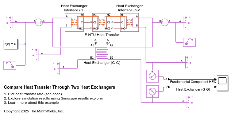
The Heat Exchanger Interface (G) block models thermal transfer by a gaseous flow within a heat exchanger. Use a second heat exchanger block to model the fluid pair. The interfaces can be in different fluid domains, such as one in liquid and one in gas. Use an E-NTU Heat Transfer block to couple the interfaces and capture the heat exchange between the fluids.

Mass Balance

The fixed-volume construction of the block allows you to capture variations in fluid mass flow rates due to compressibility. The overall mass accumulation rate is equal to the sum of the mass flow rates through the ports:

$$\dot{M}={\dot{m}}_{\text{A}}+{\dot{m}}_{\text{B}},$$

where $$\dot{M}$$ is the mass accumulation rate and $$\dot{m}$$ is the mass flow rate. The subscripts denote ports A and B. The mass flow rate is positive when it is directed into the gas channel. Variations in density are reflected in the mass accumulation rate:

$$\dot{M}=\left[{\left(\frac{\partial \rho }{\partial p}\right)}_u\frac{dp}{dt}+{\left(\frac{\partial \rho }{\partial u}\right)}_p\frac{du}{dt}\right]V,$$

where:

• ρ is density.

• p is pressure.

• u is specific internal energy.

• V is volume.

Momentum Balance

Balancing momentum between the inlet and outlet ports of the heat exchanger dictates the flow direction and speed within the exchanger. Changes in momentum are due primarily due to friction losses from pipe turns, which translate to changes in pressure. Local resistances, such as bends, elbows, and tees can result in flow separation that leads to minor additional pressure losses. For steady flows, the mass flow rate remains constant.

A momentum balance is applied to each segment of the gas (pipe) volume. This figure shows a tube bank divided into two volumes and three nodes. The nodes correspond to ports A , B, and the fluid volume, I. Fluid states, such as pressure and temperature, and fluid properties, such as density and viscosity, are defined at these nodes.

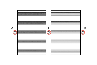
Note that flow inertia is negligible and the flow is considered to be quasi-steady state. The translation of transients to mass flow rates can be offset: due to coupling between density, pressure, and temperature, propagation of changes throughout the system is not instantaneous. Other sources and sinks of momentum, such as differences in head between ports or radial deformations of the channel wall, are not considered. The momentum balance for the half volume at port A is:

$$p_{\text{A}}-p_{\text{I}}=\Delta p_{\text{f,A}},$$

where p is the pressure at the node indicated in the subscript. Δp_f,A is the total pressure loss between the port node and the internal node due to friction. The total pressure loss includes both major and minor losses. For the half volume at port B, the momentum balance is:

$$p_{\text{B}}-p_{\text{I}}=\Delta p_{\text{f,B}}.$$

Friction

Pressure changes due to friction vary with the square of the mass flow rate for turbulent flows and with the magnitude of the mass flow rate for laminar flows. This pressure change is characterized by three dimensionless parameters: the Darcy friction factor, the pressure loss coefficient, and the Euler number. These numbers are calculated from empirical correlations or are estimated from lookup tables, depending on the Pressure loss model parameter.

Classification of "laminar" or "turbulent" flow is based on the Reynolds number. When the Reynolds number is above the Turbulent flow lower Reynolds number limit parameter, the flow is fully turbulent. Below the Laminar flow upper Reynolds number limit parameter, the flow is fully laminar. Reynolds numbers in between these values indicate transitional flow. Transitional flows show characteristics of both laminar and turbulent flows. In the Simscape™ Fluids™ language, numerical blending is applied between these bounding values.

Correlation for flow inside tubes

For tubes, the Darcy friction factor, f_D, is used. In the half volume at port A, the momentum balance is:

$$p_A-p_{\text{I}}=\frac{f_{\text{D,A}}{\dot{m}}_{\text{A}}\left|{\dot{m}}_{\text{A}}\right|}{2{\rho }_{\text{A}}{D}_{\text{H}}{A}_{\text{Min}}^2}\left(\frac{L+L_{\text{Add}}}{2}\right),$$

where L is the tube length and L_Add is the added tube length that would reproduce the minor viscous losses if used in place of elbows, tees, unions, or other local resistances. A is the tube cross-sectional area; in the event of a non-uniform cross-sectional area, A_min should be used. D_H is the tube hydraulic diameter, or the diameter of a circle equal in area to the tube cross section:

$$D_{\text{H}}=\sqrt{\frac{4A_{\text{Min}}}{\pi }}.$$

If the tube has a circular cross section, the hydraulic diameter and the tube diameter are the same.

For the half volume at port B, the momentum balance is:

$$p_{\text{B}}-p_{\text{I}}=\frac{f_{\text{D,B}}{\dot{m}}_{\text{B}}\left|{\dot{m}}_{\text{B}}\right|}{2{\rho }_{\text{B}}{D}_{\text{H}}{A}_{\text{Min}}^2}\left(\frac{L+L_{\text{Add}}}{2}\right).$$

For turbulent flows, the Darcy friction factor is calculated with the Haaland correlation. The Reynolds number is established at the bounding port:

$$f_{\text{D}}={\left\{-1.8{\text{log}}_{\text{10}}\left[\frac{6.9}{\text{Re}}+{\left(\frac{{ϵ}_{\text{R}}}{3.7D_{\text{H}}}\right)}^{1.11}\right]\right\}}^{\text{-2}},$$

where ε_R is wall roughness, taken as a characteristic height. This parameter is specified in the Internal surface absolute roughness parameter.

For laminar flows, the friction factor depends on the tube shape and is calculated with the tube shape factor:

$$f_{\text{D}}=\frac{\lambda }{\text{Re}},$$

where λ is the shape factor. The Reynolds number is calculated at the bounding port as:

$$\text{Re}=\frac{D_{\text{H}}\dot{m}}{\mu A_{\text{Min}}}.$$

Substituting Re into the pressure loss equation at port A, the momentum balance is reformulated as:

$$p_{\text{A}}-p_{\text{I}}=\frac{{\lambda }_{\text{A}}{\mu }_{\text{A}}{\dot{m}}_{\text{A}}}{2{\rho }_{\text{A}}{D}_{\text{H}}^2{A}_{\text{Min}}}\left(\frac{L+L_{\text{Add}}}{2}\right),$$

Likewise, for the half volume at port B, the momentum balance is:

$$p_{\text{B}}-p_{\text{I}}=\frac{{\lambda }_{\text{B}}{\mu }_{\text{B}}{\dot{m}}_{\text{B}}}{2{\rho }_{\text{B}}{D}_{\text{H}}^2{A}_{\text{Min}}}\left(\frac{L+L_{\text{Add}}}{2}\right).$$

Using the pressure loss coefficient

For channels other than tubes, use the pressure loss coefficient, ξ. For turbulent flows in the half volume at port A, the momentum balance is:

$$p_{\text{A}}-p_{\text{I}}=\frac{1}{2}\xi \frac{{\dot{m}}_{\text{A}}\left|{\dot{m}}_{\text{A}}\right|}{2{\rho }_{\text{A}}{A}_{\text{Min}}^2},$$

For turbulent flows in the half volume at port B, the momentum balance is:

$$p_{\text{B}}-p_{\text{I}}=\frac{1}{2}\xi \frac{{\dot{m}}_{\text{B}}\left|{\dot{m}}_{\text{B}}\right|}{2{\rho }_{\text{B}}{A}_{\text{Min}}^2},$$

For laminar flows in the half volume at port A, the momentum balance is:

$$p_{\text{A}}-p_{\text{I}}=\frac{1}{2}\xi {\text{Re}}_{\text{L}}\frac{{\dot{m}}_{\text{A}}{\mu }_{\text{A}}}{2D_{\text{H}}{\rho }_{\text{A}}{A}_{\text{Min}}},$$

where Re_L is the Laminar flow upper Reynolds number limit block parameter. For laminar flows in the half volume at port B, the momentum balance is:

$$p_{\text{B}}-p_{\text{I}}=\frac{1}{2}\xi {\text{Re}}_{\text{L}}\frac{{\dot{m}}_{\text{B}}{\mu }_{\text{B}}}{2D_{\text{H}}{\rho }_{\text{B}}{A}_{\text{Min}}}$$

Using Tabulated data - Darcy friction factor vs. Reynolds number

You can use tabulated data to determine the Darcy friction factor based on the Reynolds number for tube flows. For the half volume at port A, the momentum balance is:

$$p_{\text{A}}-p_{\text{I}}=\frac{f_{\text{D,A}}{\dot{m}}_{\text{A}}\left|{\dot{m}}_{\text{A}}\right|}{2{\rho }_{\text{A}}{D}_{\text{H}}{A}_{\text{Min}}^2}\left(\frac{L+L_{\text{Add}}}{2}\right).$$

For the half volume at port B, the momentum balance is:

$$p_{\text{B}}-p_{\text{I}}=\frac{f_{\text{D,B}}{\dot{m}}_{\text{B}}\left|{\dot{m}}_{\text{B}}\right|}{2{\rho }_{\text{B}}{D}_{\text{H}}{A}_{\text{Min}}^2}\left(\frac{L+L_{\text{Add}}}{2}\right).$$

For the turbulent regime, the friction factor is determined from a tabulated function of the Reynolds number:

$$f_{\text{D}}=f_{\text{D}}(\text{Re}).$$

The breakpoints of the tabulated function derive from the vector block parameters. The Reynolds number vector for Darcy friction factor parameter specifies the independent variable and the Darcy friction factor vector parameter specifies the dependent variable. Linear interpolation is applied between breakpoints. Outside of the tabulated data range, the nearest breakpoint determines the friction factor.

In the laminar regime, the friction factor is calculated from the shape factor, λ:

$$f_{\text{D}}=\frac{\lambda }{\text{Re}}.$$

Using Tabulated data - Euler number vs. Reynolds number

You can use tabulated data to determine the Euler number based on the Reynolds number. This calculation is dependent on flow regime, and the Euler number is formulated as a tabulated function of the Reynolds number:

$$\text{Eu}=\text{Eu}(\text{Re}).$$

The breakpoints in Tabulated data - Euler number vs. Reynolds number are specified by Reynolds number and Euler number vectors. The Reynolds number vector for Euler number parameter specifies the independent variables, the Reynolds numbers, and the Euler number vector parameter specifies the dependent variable, the Euler number, at each Reynolds number. Linear interpolation is used to determine values between breakpoints. Outside of the tabulated data range, the value at the nearest breakpoint is used.

For turbulent flows, the momentum balance for the half volume at port A is:

$$p_{\text{A}}-p_{\text{I}}={\text{Eu}}_{\text{A}}\frac{{\dot{m}}_{\text{A}}\left|{\dot{m}}_{\text{A}}\right|}{{\rho }_{\text{A}}{A}_{\text{Min}}^2},$$

where Eu is the Euler number at port A. For turbulent flows, the momentum balance for the half volume at port B is:

$$p_{\text{B}}-p_{\text{I}}={\text{Eu}}_{\text{A}}\frac{{\dot{m}}_{\text{B}}\left|{\dot{m}}_{\text{B}}\right|}{{\rho }_{\text{B}}{A}_{\text{Min}}^2}.$$

For laminar flow in the half volume at port A, the momentum balance is:

$$p_{\text{A}}-p_{\text{I}}={\text{Eu}}_{\text{L}}{\text{Re}}_{\text{L}}\frac{{\dot{m}}_{\text{A}}{\mu }_{\text{A}}}{4D_{\text{H}}{\rho }_{\text{A}}{A}_{\text{Min}}},$$

where Re_L is the Laminar flow upper Reynolds number limit parameter and Eu_L is the Euler number evaluated from tabulated data at that Reynolds number. For laminar flow in the half volume at port B, the momentum balance is:

$$p_{\text{B}}-p_{\text{I}}={\text{Eu}}_{\text{L}}{\text{Re}}_{\text{L}}\frac{{\dot{m}}_{\text{B}}{\mu }_{\text{B}}}{4D_{\text{H}}{\rho }_{\text{B}}{A}_{\text{Min}}},$$

Energy Balance

The energy balance within the gas volume is the sum of its flow rates across channel boundaries and the associated heat transfer. Energy can be transferred by advection at the ports and by convection at the wall. While conduction contributes to the energy balance at the ports, it is often negligible in comparison to advection. However, conduction is non-negligible in near-stationary fluids, such as when fluids are stagnant or changing direction. The energy balance equation is:

$${\dot{E}}_{\text{2P}}={\varphi }_{\text{A}}+{\varphi }_{\text{B}}+Q,$$

where:

• $$\frac{\partial U}{\partial p}$$ is the partial derivative of the internal energy of the gas volume with respect to pressure at constant temperature and volume.

• p_I is the pressure of the gas volume.

• $$\frac{\partial U}{\partial T}$$ is the partial derivative of the internal energy of the gas volume with respect to temperature at constant pressure and volume.

• T_I is the temperature of the gas volume.

• ϕ_A and ϕ_B are energy flow rates at ports A and B, respectively.

• Q is the heat transfer rate.

Advection and conduction are accounted for in ϕ, and convection is accounted for in Q. The heat transfer rate is positive when directed into the gas volume.

Heat Transfer Rate

Heat transfer between the two heat exchanger fluids occurs in multiple ways: through convection at the fluid interfaces, conduction through layers of built-up fouling, and conduction through the thickness of the wall.

Heat transfer extends beyond the gas channel and therefore requires other blocks to model the entire heat exchanger system. A second heat exchanger interface block models the second flow channel while an E-NTU Heat Transfer block models the heat flow across the wall. Heat transfer parameters that are specific to the gas channel, but required by the E-NTU Heat Transfer block, are available through the physical signal ports:

• Port C outputs the heat capacity rate, which is a measure of the gas' ability to absorb heat and is required for calculating the number of heat transfer units (NTU). The heat capacity rate is calculated as:

  $$C_{\text{R}}=c_{\text{p}}\dot{m},$$

  where C_R is the heat capacity rate and c_p is the specific heat.

• Port HC outputs the heat transfer coefficient, U.

  If the heat transfer coefficient is treated as a constant, its value is uniform across the flow channel. If the heat transfer coefficient is variable, it is calculated at each port from the expression:

  $$U=\frac{\text{Nu}k}{D_{\text{H,Q}}},$$

  where Nu is Nusselt number, k is thermal conductivity, and D_H,Q is a hydraulic diameter for heat transfer. The hydraulic diameterD_H,Q is calculated as:

  $$D_{\text{H,Q}}=\frac{4A_{\text{Min}}{L}_{\text{Q}}}{S_{\text{Q}}},$$

  where S_Q is the Heat transfer surface area parameter and L_Q is the Length of flow path for heat transfer parameter.

  The lower bound of the mean heat transfer coefficient is the Minimum gas-wall heat transfer coefficient parameter.

Nusselt Number

The Nusselt number is derived from empirical correlations with the Reynolds and Prandtl numbers. Use the Heat transfer parametrization parameter to select the most appropriate formulation for your simulation.

The simplest parameterization, Constant heat transfer coefficient, obtains the heat transfer coefficient directly from the value of the Gas-wall heat transfer coefficient parameter. Correlation for flow inside tubes uses analytical expressions with constant or calculated parameters to capture Nusselt number dependence on the flow regime for tube flows.

The remaining parameterizations are tabulated functions of the Reynolds number. These are useful for varying Nusselt numbers, or heat transfer coefficients, across flow regimes. The functions are generated from experimental data relating the Reynolds number to the Colburn factor or the Reynolds and Prandtl numbers to the Nusselt number.

Constant heat transfer coefficient

Using Constant heat transfer coefficient, specified in the Gas-wall heat transfer coefficient parameter, sets the heat transfer coefficient as a constant, and does not use the Nusselt number in calculations. Use this parameterization as a simple approximation for gas flows confined to the laminar regime.

Correlation for tubes

The Nusselt number depends on flow regime when using Correlation for tubes. For turbulent flows, its value changes in proportion to the Reynolds number and is calculated from the Gnielinski correlation:

$$\text{Nu}=\frac{\frac{f}{8}(\text{Re}-1000)\text{Pr}}{1+12.7\sqrt{\frac{f}{8}({\text{Pr}}^{2/3}-1)}},$$

where Re is the Reynolds number, Nu is the Nusselt number, and Pr is the Prandtl number. The friction factor, f, is the same as the factor used in tube pressure loss calculations. For laminar flows, the Nusselt number is a constant. Its value is obtained from the Nusselt number for laminar flow heat transfer parameter, Nu_L:

$$\text{Nu}={\text{Nu}}_{\text{L}}.$$

Using Tabulated data - Colburn factor vs. Reynolds number

You can use tabulated data to determine the Colburn factor based on the Reynolds number. The Colburn equation is used to determine the Nusselt number, which varies in proportion to the Reynolds number. The Colburn j-factor is a measure of proportionality between the Reynolds, Prandtl, and Nusselt numbers:

$$\text{Nu}=j({\text{Re}}_{\text{Q}}){\text{Re}}_{\text{Q}}{\text{Pr}}^{1/3}.$$

Re_Q is the Reynolds number based on the hydraulic diameter for heat transfer, D_{H, Q}, and from the minimum free-flow area of the channel, A_Min:

$${\text{Re}}_{\text{Q}}=\frac{\dot{m}{D}_{\text{H,Q}}}{A_{\text{Min}}\mu }$$

Using Tabulated data - Nusselt number vs. Reynolds number and Prandtl number

You can use a tabulated function to determine the Nusselt number from the Prandtl and Reynolds numbers. Linear interpolation is used to determine values between breakpoints. The Nusselt number is a function of both Re and Pr, and therefore the Reynolds number vector for Nusselt number, Prandtl number vector for Nusselt number, and Nusselt number table, Nu(Re,Pr) parameters define the table breakpoints:

$$\text{Nu}=\text{Nu}({\text{Re}}_{\text{Q}},\text{Pr}).$$

The tabulated Reynolds number must be calculated using the hydraulic diameter for heat transfer, D_H,Q.

Variables

To set the priority and initial target values for the block variables prior to simulation, use the Initial Targets section in the block dialog box or Property Inspector. For more information, see Set Priority and Initial Target for Block Variables and Initial Conditions for Blocks with Finite Gas Volume.

Nominal values provide a way to specify the expected magnitude of a variable in a model. Using system scaling based on nominal values increases the simulation robustness. Nominal values can come from different sources, one of which is the Nominal Values section in the block dialog box or Property Inspector. For more information, see Modify Nominal Values for a Block Variable.

Ports

Conserving

A — Gas port

gas

Entry or exit point on the gas side of the heat exchanger.

B — Gas port

gas

Entry or exit point on the gas side of the heat exchanger.

H — Thermal boundary

thermal

Thermal boundary between the modeled fluid and the heat exchanger interface.

Input

C — Heat capacity rate

physical signal

Instantaneous value of the heat capacity rate for the gas flow, specified as a physical signal.

HC — Heat transfer coefficient

physical signal

Instantaneous value of the heat transfer coefficient between gas flow and the wall, specified as a physical signal.

Parameters

Minimum free-flow area — Cross-sectional area of flow channel at its narrowest point

0.01 m^2 (default) | scalar with units of length squared

Smallest total cross-sectional flow area between inlet and outlet. If the channel is a collection of ducts, tubes, slots, or grooves, the value of this parameter is the sum of the smallest areas at the minimum flow area point. This parameter is the area where the fluid velocity is highest. For example, if the fluid flows perpendicular to a bank of tubes, the value of this parameter is the sum of the gaps between the tubes in one cross-section where the sum of the gaps is smallest is smallest.

Hydraulic diameter — Diameter or equivalent diameter of a circular channel

0.1 m (default) | scalar with units of length

Effective inner diameter of the flow. If the diameter of the cross-section varies, the value of this parameter is the diameter at its narrowest point. For non-circular channels, the hydraulic diameter is the equivalent diameter of a circle with the same area of the existing channel.

If the channel is a collection of ducts, tubes, slots, or grooves, the gross perimeter is the sum of the perimeters in the collection. If the channel is a single pipe or tube that has a circular cross section, the hydraulic diameter is equal to the true diameter.

Gas volume — Total volume of fluid contained in flow channel

0.01 m^3 (default) | scalar with units of length squared

Total volume of the fluid contained in the gas or thermal liquid flow channel.

Laminar flow upper Reynolds number limit — Start of transition between laminar and turbulent regimes

2000 (default) | scalar

Start of the transition from the laminar regime to the turbulent regime. Above this number, inertial forces become increasingly dominant. The default value is given for circular pipes and tubes with smooth surfaces.

Turbulent flow lower Reynolds number limit — End of transition between laminar and turbulent regimes

4000 (default) | scalar

End of the transition from the laminar regime to the turbulent regime. Below this number, viscous forces become increasingly dominant. The default value is for circular pipes and tubes with smooth surfaces.

Pressure loss model — Mathematical model for pressure loss due to friction

Pressure loss coefficient (default) | Correlation for flow inside tubes | Tabulated data - Darcy friction factor vs. Reynolds number | Tabulated data - Euler number vs. Reynolds number

Mathematical model for pressure loss due to friction. This setting determines which expressions to use for calculation and which block parameters to specify as input. See the Heat Exchanger Interface (TL) blocks for the calculations by parameterization.

Pressure loss coefficient — Aggregate loss coefficient for all flow resistances between the ports

0.1 (default) | scalar

Aggregate loss coefficient for all flow resistances in the flow channel, including wall friction (major losses) and local resistances due to bends, elbows, and other geometry changes (minor losses).

The loss coefficient is an empirical, dimensionless number used to express the pressure losses due to friction. It can be calculated from experimental data or obtained from product data sheets.

Dependencies

To enable this parameter, set Pressure loss model to Pressure loss coefficient.

Length of flow path from inlet to outlet — Distance traveled from port to port

1 m (default) | scalar with units of length

Total distance the flow must travel between the ports. In multi-pass shell-and-tube exchangers, the total distance is the sum over all shell passes. In tube bundles, corrugated plates, and other channels where the flow is split into parallel branches, it is the distance covered in a single branch. The longer the flow path, the steeper the major pressure loss due to friction at the wall.

Dependencies

To enable this parameter, set Pressure loss model to Correlation for flow inside tubes or Tabulated data - Darcy friction factor vs Reynolds number.

Aggregate equivalent length of local resistances — Aggregate minor pressure loss expressed in length

0.1 m (default) | scalar with units of length

Aggregate minor pressure loss, expressed as a length. The length of a straight channel results in equivalent losses to the sum of existing local resistances from elbows, tees, and unions. The larger the equivalent length, the steeper the minor pressure loss due to the local resistances.

Dependencies

To enable this parameter, set Pressure loss model to Correlation for flow inside tubes.

Internal surface absolute roughness — Mean height of wall surface variations that contribute to frictional losses

15e-6 m (default) | scalar with units of length

Mean height of the wall surface variations that contribute to frictional losses. The greater the mean height, the rougher the wall and the larger the pressure loss due to friction. Surface roughness is required to derive the Darcy friction factor from the Haaland correlation.

Dependencies

To enable this parameter, set Pressure loss model to Correlation for flow inside tubes.

Laminar friction constant for Darcy friction factor — Pressure loss correction for flow cross section in laminar flow conditions

64 (default) | scalar

Pressure loss correction for laminar flow. This parameter is referred to as the shape factor, and can be used to derive the Darcy friction factor for pressure loss calculations in the laminar regime. The default value is for cylindrical pipes and tubes.

Some additional shape factors for non-circular cross-sections can be determined from analytical solutions to the Navier-Stokes equations. A square duct has a shape factor of 56, a rectangular duct with an aspect ratio of 2:1 has a shape factor of 62, and an annular tube has a shape factor of 96. A slender conduit between parallel plates also has a shape factor of 96.

Dependencies

To enable this parameter, set Pressure loss model to Correlation for flow inside tubes.

Reynolds number vector for Darcy friction factor — Reynolds number at each breakpoint in Darcy friction factor lookup table

numerical array

Reynolds number at each breakpoint in the lookup table for the Darcy friction factor. The block interpolates between and extrapolates from the breakpoints to obtain the Darcy friction factor at any Reynolds number. Interpolation is handled by the MATLAB^® linear estimator and extrapolation is handled by the nearest function.

The Reynolds numbers must be greater than zero and increase monotonically from left to right. They can span across laminar, transient, and turbulent regimes. The number of values in this vector must be equal to the size of the Darcy friction factor vector parameter to calculate tabulated breakpoints.

Dependencies

To enable this parameter, set Pressure loss model to Tabulated data - Darcy friction factor vs. Reynolds number.

Darcy friction factor vector — Darcy friction factor at each breakpoint in Reynolds number lookup table

numerical array

Darcy friction factor at each breakpoint in the lookup table of Reynolds numbers. The block interpolates between and extrapolates from the breakpoints to obtain the Darcy friction factor at any Reynolds number. Interpolation is handled by the MATLAB linear estimator and extrapolation is handled by the nearest function.

The Darcy friction factor must not be negative and must align from left to right in order of increasing Reynolds number. The number of values in this vector must be equal to the size of the Reynolds number vector for Darcy friction factor parameter to calculate tabulated breakpoints.

Dependencies

To enable this parameter, set Pressure loss model to Tabulated data - Darcy friction factor vs. Reynolds number.

Reynolds number vector for Euler number — Reynolds number at each breakpoint in the Euler number lookup table

numerical array

Reynolds number at each breakpoint in the Euler number lookup table. The block interpolates between and extrapolates from the breakpoints to obtain the Reynolds number at any Euler number. Interpolation is handled by the MATLAB linear estimator and extrapolation is handled by the nearest function.

The Reynolds numbers must be greater than zero and increase monotonically from left to right. They can span across laminar, transient, and turbulent regimes. The number of values in this vector must be equal to the size of the Euler number vector parameter to calculate tabulated breakpoints.

Dependencies

To enable this parameter, set Pressure loss model to Tabulated data - Euler number vs. Reynolds number.

Euler number vector — Euler number at each breakpoint in the Reynolds number lookup table

numerical array

Euler number at each breakpoint in the Reynolds number lookup table. The block interpolates between and extrapolates from the breakpoints to obtain the Euler number at any Reynolds number. Interpolation is handled by the MATLAB linear estimator and extrapolation is handled by the nearest function.

The Euler number must not be negative and must align from left to right in order of increasing Reynolds number. The number of values in this vector must be equal to the size of the Reynolds number vector for Euler number parameter to calculate tabulated breakpoints.

Dependencies

To enable this parameter, set Pressure loss model to Tabulated data - Euler number vs. Reynolds number.

Heat transfer coefficient model — Mathematical model for heat transfer between fluid and wall

Constant heat transfer coefficient (default) | Correlation for flow inside tubes | Tabulated data - Colburn factor vs. Reynolds number | Tabulated data - Nusselt number vs. Reynolds number and Prandtl number

Mathematical model for heat transfer between the fluid and the wall. The choice of model determines which expressions to apply and which parameters to specify for heat transfer calculations. See the E-NTU Heat Transfer block for the calculations by parameterization.

Gas-wall heat transfer coefficient — Heat transfer coefficient for convection between fluid and wall

100 W/(m^2 * K) (default) | scalar

Heat transfer coefficient for convection between the fluid and the wall.

Dependencies

To enable this parameter, set Heat transfer coefficient model to Constant heat transfer coefficient.

Heat transfer surface area — Effective surface area used in heat transfer between fluid and wall

0.4 m^2 (default) | scalar with units of length squared

Effective surface area used in heat transfer between the fluid and the wall. The effective surface area is the sum of primary and secondary surface areas, the area where the wall is exposed to fluid and the fins, if any are used. Fin surface area is normally scaled by a fin efficiency factor.

Length of flow path for heat transfer — Characteristic length traversed in heat transfer between fluid and wall

1 m (default) | scalar with units of length

Characteristic length for heat transfer between fluid and wall. This length is used to determine the channel hydraulic diameter.

Dependencies

To enable this parameter, set Heat transfer coefficient model to Tabulated data - Colburn factor vs. Reynolds number or Tabulated data - Nusselt number vs. Reynolds number and Prandtl number.

Nusselt number for laminar flow heat transfer — Constant assumed for Nusselt number in laminar flow

3.66 (default) | positive scalar

Constant value of the Nusselt number for laminar flows. The Nusselt number is required to calculate the heat transfer coefficient between the fluid and the wall. The default value is for cylindrical pipes and tubes.

Dependencies

To enable this parameter, set Heat transfer coefficient model to Correlation for flow inside tubes.

Reynolds number vector for Colburn factor — Reynolds number at each breakpoint in Colburn factor lookup table

numerical array

Reynolds number at each breakpoint in the Colburn factor lookup table. The block interpolates between and extrapolates from the breakpoints to obtain the Colburn factor at any Reynolds number. Interpolation is handled by the MATLAB linear estimator and extrapolation is handled by the nearest function.

The Reynolds numbers must be greater than zero and increase monotonically from left to right. They can span across laminar, transient, and turbulent regimes. The number of values in this vector must be equal to the size of the Colburn factor vector parameter to calculate tabulated breakpoints.

Dependencies

To enable this parameter, set Heat transfer coefficient model to Tabulated data - Colburn factor vs. Reynolds number.

Colburn factor vector — Colburn factor at each breakpoint in Reynolds number lookup table

numerical array

The Colburn factor at each breakpoint in the Reynolds number lookup table. The block interpolates between and extrapolates from the breakpoints to obtain the Colburn factor at any Reynolds number. Interpolation is handled by the MATLAB linear estimator and extrapolation is handled by the nearest function.

The Colburn factor must be zero or positive and align from left to right in order of increasing Reynolds number. The number of values in this vector must be equal to the size of the Reynolds number vector for Colburn factor parameter to calculate tabulated breakpoints.

Dependencies

To enable this parameter, set Heat transfer coefficient model to Tabulated data - Colburn factor vs. Reynolds number.

Reynolds number vector for Nusselt number — Reynolds number at each breakpoint in Nusselt number lookup table

numerical array

The Reynolds number at each breakpoint in the Nusselt number lookup table. Either the Reynolds number or the Prandtl number can serve as an independent variable. The block interpolates between and extrapolates from the breakpoints to obtain the Nusselt number at any Reynolds number. Interpolation is handled by the MATLAB linear estimator and extrapolation is handled by the nearest function.

The Reynolds numbers must be greater than zero and increase monotonically from left to right. They can span across laminar, transient, and turbulent regimes. The size of the vector must equal the number of rows in the Nusselt number table, Nu(Re,Pr) parameter. If the table has m rows and n columns, the Reynolds number vector must be m elements long.

Dependencies

To enable this parameter, set Heat transfer coefficient model to Tabulated data - Nusselt number vs. Reynolds number and Prandtl number.

Prandtl number vector for Nusselt number — Prandtl number at each breakpoint in the Nusselt number lookup table

numerical array

Prandtl number at each breakpoint in the Nusselt number lookup table. Either the Prandtl number or the Reynolds number can serve as an independent variable. The block interpolates between and extrapolates from the breakpoints to obtain the Nusselt number at any Prandtl number. Interpolation is handled by the MATLAB linear estimator and extrapolation is handled by the nearest function.

The Prandtl number must be greater than zero and increase monotonically from left to right. They can span across laminar, transient, and turbulent regimes. The size of the vector must equal the number of columns in the Nusselt number table parameter. If the table has m rows and n columns, the Prandtl number vector must be n elements long.

Dependencies

To enable this parameter, set Heat transfer coefficient model to Tabulated data - Nusselt number vs. Reynolds number and Prandtl number.

Nusselt number table, Nu(Re,Pr) — Nusselt number at each breakpoint in Reynolds-Prandtl number lookup table

numerical array

The Nusselt number at each breakpoint in the Reynolds-Prandtl number lookup table. The block interpolates between and extrapolates from the breakpoints to obtain the Nusselt number at any pair of Reynolds and Prandtl numbers. The Nusselt number is required to calculate the heat transfer coefficient.

The Nusselt number must be greater than zero. Each value must align from top to bottom in order of increasing Reynolds number and from left to right in order of increasing Prandtl number. The number of rows must equal the size of the Reynolds number vector for Nusselt number parameter, and the number of columns must equal the size of the Prandtl number vector for Nusselt number parameter.

Dependencies

To enable this parameter, set Heat transfer coefficient model to Tabulated data - Nusselt number vs. Reynolds number and Prandtl number.

Threshold mass flow rate for flow reversal — Upper bound of numerically smooth region for mass flow rate

1e-4 kg/s (default) | scalar with units of mass per unit time

The mass flow rate below which numerical smoothing is applied. This is employed to avoid discontinuity during flow stagnation. See the Specific Dissipation Heat Exchanger Interface (G) block for more information about these calculations.

Extended Capabilities

C/C++ Code Generation
Generate C and C++ code using Simulink® Coder™.

Version History

Introduced in R2019a